Table of Contents

• 1  Data Description
• 2  Business Problem
• 3  Imports
• 4  Useful Scripts
• 5  Load the data
• 6  Preprocessing
  • 6.1  Class Balance
  • 6.2  Correlation with target
  • 6.3  Distribution plots
• 7  Scaling
  • 7.1  Outliers Removal
  • 7.2  StratifiedKFold splitting for imbalanced data
  • 7.3  Check for nans before modelling
• 8  Modelling LR with Imbalanced Data
  • 8.1  Plain Logistic Regression
  • 8.2  Grid Search for Logistic Regression
• 9  Modelling LR with Undersampling Balanced Data
  • 9.1  Plain Logistic Regression for Undersampling
  • 9.2  Logistic Regression Train on Undersample, Test in Imbalanced
  • 9.3  Grid Search for Logistic Regression with Undersampling
• 10  Modelling LR with Oversampling SMOTE
  • 10.1  oversampling using SMOTE during cross validattion using Logistic Regression
  • 10.2  Train Oversample SMOTE, Test Imbalanced
  • 10.3  Oversample SMOTE With Grid Search
  • 10.4  Polynomial Regression Train SMOTE, Test Imbalanced
    • 10.4.1  Serialize the model object and dump to a file
• 11  Model Evaluation Metrics
  • 11.1  Scalar Classification Metrics
  • 11.2  Classification Report
  • 11.3  Confusion Matrix
  • 11.4  Area Under ROC
  • 11.5  Interactive model evaluation plots

Kernel Author:
Bhishan Poudel, Data Scientist, Ph.D Astrophysics .

Data Description

The datasets contains transactions made by credit cards in September 2013 by european cardholders.

This dataset presents transactions that occurred in two days, where we have 492 frauds out of 284,807 transactions.

The dataset is highly unbalanced, the positive class (frauds) account for 0.172% of all transactions.

It contains only numerical input variables which are the result of a PCA transformation.

Unfortunately, due to confidentiality issues, we cannot provide the original features and more background information about the data.

Features V1, V2, ... V28 are the principal components obtained with PCA, the only features which have not been transformed with PCA are 'Time' and 'Amount'.

Feature 'Time' contains the seconds elapsed between each transaction and the first transaction in the dataset. The feature 'Amount' is the transaction Amount, this feature can be used for example-dependant cost-senstive learning.

Feature 'Class' is the response variable and it takes value 1 in case of fraud and 0 otherwise.

Business Problem

Business Problem:
Task    : Detect the fraudulent activities.
Metric : Recall
Sampling: Synthetic Minority Over-Sampling Technique (SMOTE)
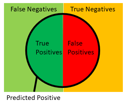
Question: How many frauds are correctly classified?

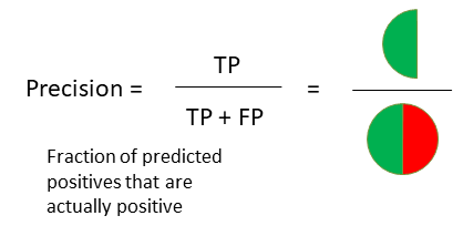
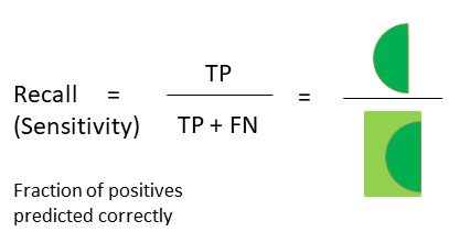
Remember that Recall = TP / (TP + FN). In case of fraud detection, classifying a fraud as non-fraud (FN) is more risky so we use the metric recall to compare the performances of the models. Higher the recall, better is the model.

The dataset is highly imbalanced. It has 284k non-frauds and 1k frauds. This means out of 1000 transatiosn, 998 are normal and 2 are fraud cases.

Also, we should note that the data is just of two days, we implicitly assume that these two days are represent of the whole trend and reflects the property of the population properly.

The could have been more or less fraudulent transactions in those particular days, but we would not take that into consideration and we generalizes the result. Or, we can say that based on the data from these two days we reached following conclusion and the result is appropriate for the population where the data distribution is similar to that of these two days.

We are more interestd in finding the Fraud cases. i.e. FN (False Negative) cases, predicting fraud as non-fraud is riskier than predicting non-fraud as fraud. So, the suitable metric of model evaluation is RECALL.

In banking, it is always the case that there are a lot of normal transactions, and only few of them are fraudulent. We may train our model with any transformation of the training data, but when testing the model the test set should look like real life, i.e., it has lots of normal cases and very few fraudulent cases.

This means we can train our model using imbalanced or balanced (undersamples or oversampled) but we should test our model on IMBALANCED dataset.

WARNINGS for Serialization:
When using the picked object (serialized object), the machine should have all the same versions of libraries used, such as numpy, pandas, scikit-learn, and all other dependency libraries.
So, to load the serialized object make sure you have the same conda environment as it was when creating the serialized object.

NOTE: When using Logistic Regression for classification problems, we have different solvers in scikit-learn such as `liblinear`, `lbfgs`, `sag`, `saga` and `newton-cg`.
`liblinear` only supports `l1` and `l2` penalty. and `saga` only supports `elasticnet`.

For small datasets, ‘liblinear’ is a good choice, whereas ‘sag’ and ‘saga’ are faster for large ones.
For multiclass problems, only ‘newton-cg’, ‘sag’, ‘saga’ and ‘lbfgs’ handle multinomial loss; ‘liblinear’ is limited to one-versus-rest schemes.
‘newton-cg’, ‘lbfgs’, ‘sag’ and ‘saga’ handle L2 or no penalty
‘liblinear’ and ‘saga’ also handle L1 penalty
‘saga’ also supports ‘elasticnet’ penalty
‘liblinear’ does not handle no penalty.

Imports

import bhishan

from bhishan.util_model_eval import get_binary_classification_scalar_metrics
from bhishan.util_model_eval import get_binary_classification_report
from bhishan.util_model_eval import print_confusion_matrix_frauds
from bhishan.util_model_eval import plot_confusion_matrix_plotly
from bhishan.util_model_eval import plot_roc_skf

%load_ext autoreload

%autoreload 2

from bhishan.util_model_eval import get_binary_classification_scalar_metrics
from bhishan.util_model_eval import print_confusion_matrix_frauds
from bhishan.util_model_eval import plot_confusion_matrix_plotly

import numpy as np
import pandas as pd
import seaborn as sns
sns.set(color_codes=True)

import matplotlib
import matplotlib.pyplot as plt
%matplotlib inline

import os
import time

# random state
SEED = 0
RNG = np.random.RandomState(SEED)

# Jupyter notebook settings for pandas
pd.set_option('display.max_columns', 200)
pd.set_option('display.max_rows', 100) # None for all the rows
pd.set_option('display.max_colwidth', 50)

print([(x.__name__,x.__version__) for x in [np, pd,sns,matplotlib]])

[('numpy', '1.16.4'), ('pandas', '0.25.0'), ('seaborn', '0.9.0'), ('matplotlib', '3.1.1')]

import scipy
from scipy import stats

# six and pickle
import six
import pickle
import joblib

# scale and split
from sklearn.preprocessing import MinMaxScaler, StandardScaler, RobustScaler
from sklearn.model_selection import train_test_split
from sklearn.model_selection import StratifiedKFold

# classifiers
from sklearn.linear_model import LogisticRegression

# grid search
from sklearn.model_selection import GridSearchCV, RandomizedSearchCV
from sklearn.model_selection import StratifiedKFold

# pipeline
from sklearn.pipeline import make_pipeline
from imblearn.pipeline import make_pipeline as imbalanced_make_pipeline

/Users/poudel/miniconda3/envs/dataSc/lib/python3.7/site-packages/sklearn/externals/six.py:31: DeprecationWarning: The module is deprecated in version 0.21 and will be removed in version 0.23 since we've dropped support for Python 2.7. Please rely on the official version of six (https://pypi.org/project/six/).
  "(https://pypi.org/project/six/).", DeprecationWarning)

# smote
from imblearn.over_sampling import SMOTE
from imblearn.metrics import classification_report_imbalanced
from imblearn.pipeline import make_pipeline as imbalanced_make_pipeline

# sklearn scalar metrics
from sklearn.metrics import accuracy_score
from sklearn.metrics import precision_score
from sklearn.metrics import recall_score
from sklearn.metrics import f1_score

# multiple metrics
from sklearn.metrics import average_precision_score
from sklearn.metrics import precision_recall_fscore_support

# roc auc and curves
from sklearn.metrics import auc
from sklearn.metrics import roc_auc_score
from sklearn.metrics import roc_curve
from sklearn.metrics import precision_recall_curve

# confusion matrix and classification report
from sklearn.metrics import confusion_matrix
from sklearn.metrics import classification_report

Useful Scripts

def show_method_attributes(method, ncols=7,exclude=None):
    """ Show all the attributes of a given method.
    Example:
    ========
    show_method_attributes(list)
     """
    x = [I for I in dir(method) if I[0]!='_' ]
    x = [I for I in x 
         if I not in 'os np pd sys time psycopg2'.split()
         if (exclude not in i)
        ]
             

    return pd.DataFrame(np.array_split(x,ncols)).T.fillna('')

Load the data

df = pd.read_csv('../data/raw/creditcard.csv.zip',compression='zip')
print(df.shape)
df.head()

(284807, 31)

	Time	V1	V2	V3	V4	V5	V6	V7	V8	V9	V10	V11	V12	V13	V14	V15	V16	V17	V18	V19	V20	V21	V22	V23	V24	V25	V26	V27	V28	Amount	Class
0	0.0	-1.359807	-0.072781	2.536347	1.378155	-0.338321	0.462388	0.239599	0.098698	0.363787	0.090794	-0.551600	-0.617801	-0.991390	-0.311169	1.468177	-0.470401	0.207971	0.025791	0.403993	0.251412	-0.018307	0.277838	-0.110474	0.066928	0.128539	-0.189115	0.133558	-0.021053	149.62	0
1	0.0	1.191857	0.266151	0.166480	0.448154	0.060018	-0.082361	-0.078803	0.085102	-0.255425	-0.166974	1.612727	1.065235	0.489095	-0.143772	0.635558	0.463917	-0.114805	-0.183361	-0.145783	-0.069083	-0.225775	-0.638672	0.101288	-0.339846	0.167170	0.125895	-0.008983	0.014724	2.69	0
2	1.0	-1.358354	-1.340163	1.773209	0.379780	-0.503198	1.800499	0.791461	0.247676	-1.514654	0.207643	0.624501	0.066084	0.717293	-0.165946	2.345865	-2.890083	1.109969	-0.121359	-2.261857	0.524980	0.247998	0.771679	0.909412	-0.689281	-0.327642	-0.139097	-0.055353	-0.059752	378.66	0
3	1.0	-0.966272	-0.185226	1.792993	-0.863291	-0.010309	1.247203	0.237609	0.377436	-1.387024	-0.054952	-0.226487	0.178228	0.507757	-0.287924	-0.631418	-1.059647	-0.684093	1.965775	-1.232622	-0.208038	-0.108300	0.005274	-0.190321	-1.175575	0.647376	-0.221929	0.062723	0.061458	123.50	0
4	2.0	-1.158233	0.877737	1.548718	0.403034	-0.407193	0.095921	0.592941	-0.270533	0.817739	0.753074	-0.822843	0.538196	1.345852	-1.119670	0.175121	-0.451449	-0.237033	-0.038195	0.803487	0.408542	-0.009431	0.798278	-0.137458	0.141267	-0.206010	0.502292	0.219422	0.215153	69.99	0

Preprocessing

Class Balance

df['Class'].value_counts()

0    284315
1       492
Name: Class, dtype: int64

df['Class'].value_counts(normalize=True)*1000

0    998.272514
1      1.727486
Name: Class, dtype: float64

Correlation with target

target = 'Class'
df_corr = df.drop(target,1).corrwith(df[target]).sort_values()

df_corr.plot.bar(figsize = (12, 8), title = "Correlation with class",
          fontsize = 12,rot = 90, grid = True,
          color=sns.color_palette('Reds_r',30),ylim=(-0.4,0.4)
       )

# v17 14 12 and 10 has correlation more than 0.2

<matplotlib.axes._subplots.AxesSubplot at 0x10b39f5c0>

Distribution plots

df_corr.loc[ abs(df_corr.values)>0.2]

V17   -0.326481
V14   -0.302544
V12   -0.260593
V10   -0.216883
dtype: float64

high_corr_idx = df_corr.loc[ abs(df_corr.values)>0.2].index.values.tolist()
high_corr_idx

['V17', 'V14', 'V12', 'V10']

def dist_plot():
    for c in high_corr_idx:
        sns.distplot(df[c],fit=scipy.stats.norm)
        plt.xlim(-5,5)
        plt.show()
        plt.close()
        
# dist_plot()

# clearly pdf is much different from gaussian distribution.
# to reduce skewness, we can we boxcox transform.

Scaling

# RobustScaler is less prone to outliers.
from sklearn.preprocessing import StandardScaler, RobustScaler

scaler = RobustScaler()

df['scaled_amount'] = scaler.fit_transform(df['Amount'].values.reshape(-1,1))
df['scaled_time'] = scaler.fit_transform(df['Time'].values.reshape(-1,1))

Outliers Removal

def boxplots_with_outliers():
    print('Before removing outliers from highest correlated features:')
    for c in high_corr_idx:
        plt.figure(figsize=(16,4))
        sns.boxplot(df[c])
        plt.show()
        plt.close()

# boxplots_with_outliers()

# Find outliers using IQR method
q1 = df[high_corr_idx].quantile(0.25)
q3 = df[high_corr_idx].quantile(0.75)
iqr = q3 - q1
threshold = 1.5

cond1 = df[high_corr_idx] < (q1 - threshold * iqr)
cond2 = df[high_corr_idx] > (q3 + threshold * iqr)
cond = cond1 | cond2

idx_no_outliers = df[high_corr_idx][~(cond).any(axis=1)].index
idx_no_outliers[:5]

Int64Index([0, 1, 2, 3, 4], dtype='int64')

df_no_outliers = df.loc[idx_no_outliers]

df.shape, df_no_outliers.shape

((284807, 33), (250883, 33))

def boxplots_no_outliers():
    print('After removing outliers from highest correlated features:')
    for c in high_corr_idx:
        plt.figure(figsize=(16,4))
        sns.boxplot(df_no_outliers[c])
        plt.show()
        plt.close()
        
# boxplots_no_outliers()

StratifiedKFold splitting for imbalanced data

from sklearn.model_selection import StratifiedKFold

df.columns.values

array(['Time', 'V1', 'V2', 'V3', 'V4', 'V5', 'V6', 'V7', 'V8', 'V9',
       'V10', 'V11', 'V12', 'V13', 'V14', 'V15', 'V16', 'V17', 'V18',
       'V19', 'V20', 'V21', 'V22', 'V23', 'V24', 'V25', 'V26', 'V27',
       'V28', 'Amount', 'Class', 'scaled_amount', 'scaled_time'],
      dtype=object)

target = 'Class'
features_no_log = df.columns.difference(['Amount','Time','Class']).values.tolist()
features_with_log = df.columns.difference(['scaled_amount','scaled_time','Class']).values.tolist()

idx = idx_no_outliers
cols = features_with_log

df_X = df.loc[idx,cols]
df_y = df.loc[idx,target]


skf = StratifiedKFold(n_splits=5, random_state=SEED, shuffle=True)

for idx_tr, idx_tx in skf.split(df_X, df_y):
    df_Xtrain, df_Xtest = df_X.iloc[idx_tr], df_X.iloc[idx_tx]
    df_ytrain, df_ytest = df_y.iloc[idx_tr], df_y.iloc[idx_tx]

# for imbalanced data, we use stratified k fold splitting
# class proportion are maintained same in train and test
df_ytrain.value_counts(normalize=True).append(df_ytest.value_counts(normalize=True))

0    0.999841
1    0.000159
0    0.999860
1    0.000140
Name: Class, dtype: float64

Check for nans before modelling

df.isnull().sum().sum()

0

df['Class'].value_counts()

0    284315
1       492
Name: Class, dtype: int64

Modelling LR with Imbalanced Data

# we need numpy arrays for stratified splitting.
Xtrain = df_Xtrain.values
Xtest = df_Xtest.values
ytrain = df_ytrain.values
ytest = df_ytest.values

Plain Logistic Regression

from sklearn.linear_model import LogisticRegression
from sklearn.metrics import classification_report, recall_score

# define classifer
clf_lr = LogisticRegression(solver='liblinear',
                            max_iter=4000,
                            random_state=SEED,
                            n_jobs=1) # for liblinear n_jobs is +1.

# fit the classifier
clf_lr.fit(Xtrain,ytrain)

# get the prediction
ypreds_lr = clf_lr.predict(Xtest)

# model eval
recall = recall_score(ytest,ypreds_lr)
report = classification_report(ytest,ypreds_lr)

print(f'Recall Logistic Regression {recall: .2f}')
print(report) 

# I got ZERO recall, all the frauds are classified as non-frauds
# the model overfitted since there are too many non-frauds cases.

Recall Logistic Regression  0.00
              precision    recall  f1-score   support

           0       1.00      1.00      1.00     50168
           1       0.00      0.00      0.00         7

    accuracy                           1.00     50175
   macro avg       0.50      0.50      0.50     50175
weighted avg       1.00      1.00      1.00     50175

/Users/poudel/miniconda3/envs/dataSc/lib/python3.7/site-packages/sklearn/metrics/classification.py:1437: UndefinedMetricWarning: Precision and F-score are ill-defined and being set to 0.0 in labels with no predicted samples.
  'precision', 'predicted', average, warn_for)

from bhishan.util_model_eval import get_binary_classification_scalar_metrics

df_eval = get_binary_classification_scalar_metrics(
    "Logistic Regression",
    clf_lr,
    Xtest,ytest,
    ypreds_lr,
    desc="Train Test Imbalanced", df_eval=None)

/Users/poudel/miniconda3/envs/dataSc/lib/python3.7/site-packages/sklearn/metrics/classification.py:1437: UndefinedMetricWarning: Precision is ill-defined and being set to 0.0 due to no predicted samples.
  'precision', 'predicted', average, warn_for)
/Users/poudel/miniconda3/envs/dataSc/lib/python3.7/site-packages/sklearn/metrics/classification.py:1437: UndefinedMetricWarning: F-score is ill-defined and being set to 0.0 due to no predicted samples.
  'precision', 'predicted', average, warn_for)
/Users/poudel/miniconda3/envs/dataSc/lib/python3.7/site-packages/sklearn/metrics/classification.py:872: RuntimeWarning: invalid value encountered in double_scalars
  mcc = cov_ytyp / np.sqrt(cov_ytyt * cov_ypyp)

	Model	Description	Accuracy	Precision	Recall	F1	Mathews Correlation Coefficient	Cohens Kappa	Area Under Precision Curve	Area Under ROC Curve
0	Logistic Regression	Train Test Imbalanced	0.99986	0	0	0	0	0	0.00305379	0.624277

from bhishan.util_model_eval import get_binary_classification_report

df_clf_report = get_binary_classification_report("Logistic Regression",
  ytest,
  ypreds_lr,
  desc='',
  style_col='Recall_1',
  df_clf_report=None)

/Users/poudel/miniconda3/envs/dataSc/lib/python3.7/site-packages/sklearn/metrics/classification.py:1437: UndefinedMetricWarning: Precision and F-score are ill-defined and being set to 0.0 in labels with no predicted samples.
  'precision', 'predicted', average, warn_for)

	Model	Description	Precision_0	Precision_1	Recall_0	Recall_1	F1_Score_0	F1_Score_1	Support_0	Support_1
0	Logistic Regression		0.99986	0	1	0	0.99993	0	50168	7

print(classification_report(ytest, ypreds_lr))

              precision    recall  f1-score   support

           0       1.00      1.00      1.00     50168
           1       0.00      0.00      0.00         7

    accuracy                           1.00     50175
   macro avg       0.50      0.50      0.50     50175
weighted avg       1.00      1.00      1.00     50175

/Users/poudel/miniconda3/envs/dataSc/lib/python3.7/site-packages/sklearn/metrics/classification.py:1437: UndefinedMetricWarning: Precision and F-score are ill-defined and being set to 0.0 in labels with no predicted samples.
  'precision', 'predicted', average, warn_for)

from bhishan.util_model_eval import print_confusion_matrix_frauds

print_confusion_matrix_frauds("Logistic Regression", ytest,ypreds_lr)

Logistic Regression

	Predicted_No_Fraud	Predicted_Fraud	Total_Frauds	Correct_Frauds	Incorrect_Frauds	Fraud_Detection
No_Fraud	50,168	0	7	0	7	0.00%
Fraud	7	0	7	0	7	0.00%

confusion_matrix(ytest, ypreds_lr)

array([[50168,     0],
       [    7,     0]])

from bhishan.util_model_eval import plot_confusion_matrix_plotly

# plot_confusion_matrix_plotly(ytest, ypreds_lr)

Grid Search for Logistic Regression

def do_grid_search(clf, params,Xtrain,ytrain,scoring='recall'):
    """Grid Search Cross Validation for given classifier.
    
    NOTE:
    1. Use scoring = 'recall' for fraud detection, patient detection like
       situations where FN (False Negative) is more important.
       
    2. Use scoring = 'precision' for spam email detection like cases
       where FP (False Positive) is more important.
    
    """
    from sklearn.model_selection import GridSearchCV
    
    t0 = time.time()
    grid = GridSearchCV(clf, params,cv=5,n_jobs=-1,verbose=2,scoring=scoring)
    grid.fit(Xtrain, ytrain)

    clf_best = grid.best_estimator_

    t1 = time.time() - t0
    print('Time taken: {} minutes {:.2f} seconds'.format(*divmod(t1,60)))
    
    return clf_best

# Logistic Regression with Grid search
# Time taken: 4 min 31 secs

t0 = time.time()
clf_lr_grid = LogisticRegression(solver='liblinear',
                            max_iter=4000,
                            random_state=SEED,
                            n_jobs=1) # for liblinear n_jobs is +1.

params_lr_grid = {"penalty": ['l1', 'l2'],
                  'C': [0.001, 0.01, 0.1, 1, 10, 100, 1000]}

clf_lr_grid = do_grid_search(clf_lr_grid, params_lr_grid,
                             Xtrain,ytrain)
t1 = time.time() - t0
print('Time taken: {:.0f} min {:.0f} secs'.format(*divmod(t1,60)))

Fitting 5 folds for each of 14 candidates, totalling 70 fits

[Parallel(n_jobs=-1)]: Using backend LokyBackend with 4 concurrent workers.
[Parallel(n_jobs=-1)]: Done  33 tasks      | elapsed:   29.7s
[Parallel(n_jobs=-1)]: Done  70 out of  70 | elapsed:  2.8min finished

Time taken: 2.0 minutes 46.13 seconds
Time taken: 2 min 46 secs

ypreds_lr_grid = clf_lr_grid.predict(Xtest)

recall_grid = recall_score(ytest, ypreds_lr_grid)
report_grid = classification_report(ytest,ypreds_lr_grid)

print(f'Recall LR Grid search {recall_grid: .2f}')
print(report_grid)

# Even after grid search, I got recall 0 for fraud cases.
# The model is still overfitting.
# There are 
# Some possible ways to handle this are:
#   1. random undersampling (this makes dataset about 1k from 285k)
#   2. random oversampling using SMOTE (this makes dataset about 284*2k from 285k)

Recall LR Grid search  0.00
              precision    recall  f1-score   support

           0       1.00      1.00      1.00     50168
           1       0.00      0.00      0.00         7

    accuracy                           1.00     50175
   macro avg       0.50      0.50      0.50     50175
weighted avg       1.00      1.00      1.00     50175

/Users/poudel/miniconda3/envs/dataSc/lib/python3.7/site-packages/sklearn/metrics/classification.py:1437: UndefinedMetricWarning: Precision and F-score are ill-defined and being set to 0.0 in labels with no predicted samples.
  'precision', 'predicted', average, warn_for)

df_eval = get_binary_classification_scalar_metrics(
    'Logistic Regression',
    clf_lr_grid,
    Xtest,ytest,
    ypreds_lr_grid,
    desc="Train Test Imbalanced, Grid Search", df_eval=df_eval)

/Users/poudel/miniconda3/envs/dataSc/lib/python3.7/site-packages/sklearn/metrics/classification.py:1437: UndefinedMetricWarning: Precision is ill-defined and being set to 0.0 due to no predicted samples.
  'precision', 'predicted', average, warn_for)
/Users/poudel/miniconda3/envs/dataSc/lib/python3.7/site-packages/sklearn/metrics/classification.py:1437: UndefinedMetricWarning: F-score is ill-defined and being set to 0.0 due to no predicted samples.
  'precision', 'predicted', average, warn_for)
/Users/poudel/miniconda3/envs/dataSc/lib/python3.7/site-packages/sklearn/metrics/classification.py:872: RuntimeWarning: invalid value encountered in double_scalars
  mcc = cov_ytyp / np.sqrt(cov_ytyt * cov_ypyp)

	Model	Description	Accuracy	Precision	Recall	F1	Mathews Correlation Coefficient	Cohens Kappa	Area Under Precision Curve	Area Under ROC Curve
0	Logistic Regression	Train Test Imbalanced	0.99986	0	0	0	0	0	0.00305379	0.624277
1	Logistic Regression	Train Test Imbalanced, Grid Search	0.99986	0	0	0	0	0	0.000155879	0.466225

df_clf_report = get_binary_classification_report("Logistic Regression",
  ytest,
  ypreds_lr,
  desc='Train Test Imbalanced, Grid Search',
  style_col='Recall_1',
  df_clf_report=df_clf_report)

/Users/poudel/miniconda3/envs/dataSc/lib/python3.7/site-packages/sklearn/metrics/classification.py:1437: UndefinedMetricWarning: Precision and F-score are ill-defined and being set to 0.0 in labels with no predicted samples.
  'precision', 'predicted', average, warn_for)

	Model	Description	Precision_0	Precision_1	Recall_0	Recall_1	F1_Score_0	F1_Score_1	Support_0	Support_1
0	Logistic Regression		0.99986	0	1	0	0.99993	0	50168	7
1	Logistic Regression	Train Test Imbalanced, Grid Search	0.99986	0	1	0	0.99993	0	50168	7

print(classification_report(ytest,ypreds_lr_grid ))

              precision    recall  f1-score   support

           0       1.00      1.00      1.00     50168
           1       0.00      0.00      0.00         7

    accuracy                           1.00     50175
   macro avg       0.50      0.50      0.50     50175
weighted avg       1.00      1.00      1.00     50175

/Users/poudel/miniconda3/envs/dataSc/lib/python3.7/site-packages/sklearn/metrics/classification.py:1437: UndefinedMetricWarning: Precision and F-score are ill-defined and being set to 0.0 in labels with no predicted samples.
  'precision', 'predicted', average, warn_for)

print_confusion_matrix_frauds("Train Test Imbalanced, Grid Search",
                       ytest,ypreds_lr_grid)

Train Test Imbalanced, Grid Search

	Predicted_No_Fraud	Predicted_Fraud	Total_Frauds	Correct_Frauds	Incorrect_Frauds	Fraud_Detection
No_Fraud	50,168	0	7	0	7	0.00%
Fraud	7	0	7	0	7	0.00%

confusion_matrix(ytest, ypreds_lr_grid)

array([[50168,     0],
       [    7,     0]])

Modelling LR with Undersampling Balanced Data

Plain Logistic Regression for Undersampling

target = 'Class'
n = df[target].value_counts().values[-1]

df_under = (df.groupby(target)
                .apply(lambda x: x.sample(n,random_state=SEED))
                .reset_index(drop=True)
               )

df_under[target].value_counts()

1    492
0    492
Name: Class, dtype: int64

df_under.columns

Index(['Time', 'V1', 'V2', 'V3', 'V4', 'V5', 'V6', 'V7', 'V8', 'V9', 'V10',
       'V11', 'V12', 'V13', 'V14', 'V15', 'V16', 'V17', 'V18', 'V19', 'V20',
       'V21', 'V22', 'V23', 'V24', 'V25', 'V26', 'V27', 'V28', 'Amount',
       'Class', 'scaled_amount', 'scaled_time'],
      dtype='object')

features_with_log = ['V1', 'V2', 'V3', 'V4', 'V5', 'V6', 'V7', 'V8', 'V9', 'V10',
       'V11', 'V12', 'V13', 'V14', 'V15', 'V16', 'V17', 'V18', 'V19', 'V20',
       'V21', 'V22', 'V23', 'V24', 'V25', 'V26', 'V27', 'V28', 
       'scaled_amount', 'scaled_time']

Xtrain_under,Xtest_under,ytrain_under,ytest_under = \
  train_test_split(df_under[features_with_log],
                   df_under[target],
                   test_size=0.2,
                   stratify=df_under[target],
                   random_state=SEED)

from sklearn.linear_model import LogisticRegression
from sklearn.metrics import classification_report, recall_score

# define classifer
clf_lr_under = LogisticRegression(solver='liblinear',
                            max_iter=4000,
                            random_state=SEED,
                            n_jobs=1) # for liblinear n_jobs is +1.

# fit the classifier
clf_lr_under.fit(Xtrain_under,ytrain_under)

# get the prediction
ypreds_lr_under = clf_lr_under.predict(Xtest_under) ## ** Test on Undersample**

# model eval
recall_under = recall_score(ytest_under,ypreds_lr_under)
report_under = classification_report(ytest_under,ypreds_lr_under)

print(f'Recall: Train Test Undersample {recall_under: .2f}')
print(report_under)

# Now we have much small dataset, but much better recall scores.

Recall: Train Test Undersample  0.93
              precision    recall  f1-score   support

           0       0.93      0.96      0.95        99
           1       0.96      0.93      0.94        98

    accuracy                           0.94       197
   macro avg       0.94      0.94      0.94       197
weighted avg       0.94      0.94      0.94       197

df_eval = get_binary_classification_scalar_metrics(
    'Logistic Regression',
    clf_lr_under,
    Xtest_under,ytest_under,
    ypreds_lr_under,
    desc="Train Test Undersample", df_eval=df_eval)

	Model	Description	Accuracy	Precision	Recall	F1	Mathews Correlation Coefficient	Cohens Kappa	Area Under Precision Curve	Area Under ROC Curve
0	Logistic Regression	Train Test Undersample	0.944162	0.957895	0.928571	0.943005	0.888717	0.888305	0.991175	0.989281
1	Logistic Regression	Train Test Imbalanced	0.99986	0	0	0	0	0	0.00305379	0.624277
2	Logistic Regression	Train Test Imbalanced, Grid Search	0.99986	0	0	0	0	0	0.000155879	0.466225

df_clf_report = get_binary_classification_report("Logistic Regression",
  ytest_under,
  ypreds_lr_under,
  desc='Train Test Undersample',
  style_col='Recall_1',
  df_clf_report=df_clf_report)

	Model	Description	Precision_0	Precision_1	Recall_0	Recall_1	F1_Score_0	F1_Score_1	Support_0	Support_1
2	Logistic Regression	Train Test Undersample	0.931373	0.957895	0.959596	0.928571	0.945274	0.943005	99	98
0	Logistic Regression		0.99986	0	1	0	0.99993	0	50168	7
1	Logistic Regression	Train Test Imbalanced, Grid Search	0.99986	0	1	0	0.99993	0	50168	7

print(classification_report(ytest_under,ypreds_lr_under))

              precision    recall  f1-score   support

           0       0.93      0.96      0.95        99
           1       0.96      0.93      0.94        98

    accuracy                           0.94       197
   macro avg       0.94      0.94      0.94       197
weighted avg       0.94      0.94      0.94       197

print_confusion_matrix_frauds('Train Test Undersample',
                       ytest_under,ypreds_lr_under)

Train Test Undersample

	Predicted_No_Fraud	Predicted_Fraud	Total_Frauds	Correct_Frauds	Incorrect_Frauds	Fraud_Detection
No_Fraud	95	4	98	91	7	92.86%
Fraud	7	91	98	91	7	92.86%

confusion_matrix(ytest_under,ypreds_lr_under)

array([[95,  4],
       [ 7, 91]])

Logistic Regression Train on Undersample, Test in Imbalanced

Xtest.shape, Xtest_under.shape

((50175, 30), (197, 30))

from sklearn.linear_model import LogisticRegression
from sklearn.metrics import classification_report, recall_score

# define classifer
clf_lr_under_imb = LogisticRegression(solver='liblinear',
                            max_iter=4000,
                            random_state=SEED,
                            n_jobs=1) # for liblinear n_jobs is +1.

# fit the classifier
clf_lr_under_imb.fit(Xtrain_under,ytrain_under)

# get the prediction
ypreds_lr_under_imb = clf_lr_under.predict(Xtest) ## ** Test on Imbalanced**

# model eval
recall_under_imb = recall_score(ytest,ypreds_lr_under_imb)
report_under_imb = classification_report(ytest,ypreds_lr_under_imb)

print(f'Recall: Train Underample, Test Imbalanced {recall_under_imb: .2f}')
print(report_under_imb)

# Now we have much small dataset, but much better recall scores.

Recall: Train Underample, Test Imbalanced  0.00
              precision    recall  f1-score   support

           0       1.00      1.00      1.00     50168
           1       0.00      0.00      0.00         7

    accuracy                           1.00     50175
   macro avg       0.50      0.50      0.50     50175
weighted avg       1.00      1.00      1.00     50175

df_eval = get_binary_classification_scalar_metrics(
    'Logistic Regression',
    clf_lr_under_imb,
    Xtest,ytest,
    ypreds_lr_under_imb,
    desc="Train Undersample, Test Imbalanced", df_eval=df_eval)

	Model	Description	Accuracy	Precision	Recall	F1	Mathews Correlation Coefficient	Cohens Kappa	Area Under Precision Curve	Area Under ROC Curve
0	Logistic Regression	Train Test Undersample	0.944162	0.957895	0.928571	0.943005	0.888717	0.888305	0.991175	0.989281
1	Logistic Regression	Train Test Imbalanced	0.99986	0	0	0	0	0	0.00305379	0.624277
2	Logistic Regression	Train Test Imbalanced, Grid Search	0.99986	0	0	0	0	0	0.000155879	0.466225
3	Logistic Regression	Train Undersample, Test Imbalanced	0.999482	0	0	0	-0.000229906	-0.000203943	0.000139512	0.492705

df_clf_report = get_binary_classification_report("Logistic Regression",
  ytest,
  ypreds_lr_under_imb,
  desc='Train Undersample, Test Imbalanced',
  style_col='Recall_1',
  df_clf_report=df_clf_report)

	Model	Description	Precision_0	Precision_1	Recall_0	Recall_1	F1_Score_0	F1_Score_1	Support_0	Support_1
2	Logistic Regression	Train Test Undersample	0.931373	0.957895	0.959596	0.928571	0.945274	0.943005	99	98
0	Logistic Regression		0.99986	0	1	0	0.99993	0	50168	7
1	Logistic Regression	Train Test Imbalanced, Grid Search	0.99986	0	1	0	0.99993	0	50168	7
3	Logistic Regression	Train Undersample, Test Imbalanced	0.99986	0	0.999621	0	0.999741	0	50168	7

print(classification_report(ytest,ypreds_lr_under_imb))

              precision    recall  f1-score   support

           0       1.00      1.00      1.00     50168
           1       0.00      0.00      0.00         7

    accuracy                           1.00     50175
   macro avg       0.50      0.50      0.50     50175
weighted avg       1.00      1.00      1.00     50175

print_confusion_matrix_frauds('Train Undersample, Test Undersample',
                       ytest,ypreds_lr_under_imb)

Train Undersample, Test Undersample

	Predicted_No_Fraud	Predicted_Fraud	Total_Frauds	Correct_Frauds	Incorrect_Frauds	Fraud_Detection
No_Fraud	50,149	19	7	0	7	0.00%
Fraud	7	0	7	0	7	0.00%

confusion_matrix(ytest,ypreds_lr_under_imb)

array([[50149,    19],
       [    7,     0]])

Grid Search for Logistic Regression with Undersampling

# Grid Search for Logistic Regression with Undersampling 
clf_lr_under_grid = LogisticRegression(solver='liblinear',
                            max_iter=4000,
                            random_state=SEED,
                            n_jobs=1) # for liblinear n_jobs is +1.

params_lr_under_grid = {"penalty": ['l1', 'l2'],
                  'C': [0.001, 0.01, 0.1, 1, 10, 100, 1000]}

clf_lr_under_grid = do_grid_search(clf_lr_under_grid, params_lr_under_grid,
                                   Xtrain_under,ytrain_under)

Fitting 5 folds for each of 14 candidates, totalling 70 fits

[Parallel(n_jobs=-1)]: Using backend LokyBackend with 4 concurrent workers.

Time taken: 0.0 minutes 1.97 seconds

[Parallel(n_jobs=-1)]: Done  70 out of  70 | elapsed:    2.0s finished

ypreds_lr_under_grid = clf_lr_under_grid.predict(Xtest_under)

recall_under_grid = recall_score(ytest_under, ypreds_lr_under_grid)
report_under_grid = classification_report(ytest_under,ypreds_lr_under_grid)

print(f'Recall: Train Test Undersample, Grid Search {recall_under_grid: .2f}')
print(report_under_grid)

# recall for fraud is 0.92 and for non-fraud is 0.96 for undersample only
# recall for fraud is 0.92 and for non-fraud is 0.98 for undersample grid search

Recall: Train Test Undersample, Grid Search  0.94
              precision    recall  f1-score   support

           0       0.94      0.91      0.92        99
           1       0.91      0.94      0.92        98

    accuracy                           0.92       197
   macro avg       0.92      0.92      0.92       197
weighted avg       0.92      0.92      0.92       197

df_eval = get_binary_classification_scalar_metrics(
    'Logistic Regression',
    clf_lr_under_grid,
    Xtest_under,ytest_under,
    ypreds_lr_under_grid,
    desc="Train Test Undersample, Grid Search", df_eval=df_eval)

	Model	Description	Accuracy	Precision	Recall	F1	Mathews Correlation Coefficient	Cohens Kappa	Area Under Precision Curve	Area Under ROC Curve
0	Logistic Regression	Train Test Undersample, Grid Search	0.923858	0.910891	0.938776	0.924623	0.848129	0.847735	0.985611	0.97918
1	Logistic Regression	Train Test Undersample	0.944162	0.957895	0.928571	0.943005	0.888717	0.888305	0.991175	0.989281
2	Logistic Regression	Train Test Imbalanced	0.99986	0	0	0	0	0	0.00305379	0.624277
3	Logistic Regression	Train Test Imbalanced, Grid Search	0.99986	0	0	0	0	0	0.000155879	0.466225
4	Logistic Regression	Train Undersample, Test Imbalanced	0.999482	0	0	0	-0.000229906	-0.000203943	0.000139512	0.492705

df_clf_report = get_binary_classification_report("Logistic Regression",
  ytest_under,
  ypreds_lr_under_grid,
  desc='Train Test Undersample, Grid Search',
  style_col='Recall_1',
  df_clf_report=df_clf_report)

	Model	Description	Precision_0	Precision_1	Recall_0	Recall_1	F1_Score_0	F1_Score_1	Support_0	Support_1
4	Logistic Regression	Train Test Undersample, Grid Search	0.9375	0.910891	0.909091	0.938776	0.923077	0.924623	99	98
2	Logistic Regression	Train Test Undersample	0.931373	0.957895	0.959596	0.928571	0.945274	0.943005	99	98
0	Logistic Regression		0.99986	0	1	0	0.99993	0	50168	7
1	Logistic Regression	Train Test Imbalanced, Grid Search	0.99986	0	1	0	0.99993	0	50168	7
3	Logistic Regression	Train Undersample, Test Imbalanced	0.99986	0	0.999621	0	0.999741	0	50168	7

print(classification_report(ytest_under,ypreds_lr_under_grid))

              precision    recall  f1-score   support

           0       0.94      0.91      0.92        99
           1       0.91      0.94      0.92        98

    accuracy                           0.92       197
   macro avg       0.92      0.92      0.92       197
weighted avg       0.92      0.92      0.92       197

print_confusion_matrix_frauds("Train Test Undersample, Grid Search",
                             ytest_under,ypreds_lr_under_grid)

Train Test Undersample, Grid Search

	Predicted_No_Fraud	Predicted_Fraud	Total_Frauds	Correct_Frauds	Incorrect_Frauds	Fraud_Detection
No_Fraud	90	9	98	92	6	93.88%
Fraud	6	92	98	92	6	93.88%

confusion_matrix(ytest_under,ypreds_lr_under_grid)

array([[90,  9],
       [ 6, 92]])

Modelling LR with Oversampling SMOTE

oversampling using SMOTE during cross validattion using Logistic Regression

from sklearn.model_selection import RandomizedSearchCV
from sklearn.model_selection import StratifiedKFold
from imblearn.pipeline import make_pipeline as imbalanced_make_pipeline
from imblearn.over_sampling import SMOTE
from sklearn.linear_model import LogisticRegression
import time

# Overampling and cross validation

def modelling_smote_lr_cross_validation(fname_pkl):
    import io
    import joblib
    # Time taken 45.0 mins 55.83 seconds

    t0 = time.time()

    # metrics lists
    accuracy_lst, precision_lst,recall_lst,f1_lst,auc_lst = [], [], [], [], []

    # randomized classifier
    clf_lr_params = {"penalty": ['l1', 'l2'],
                      'C': [0.001, 0.01, 0.1, 1, 10, 100, 1000]
                    }

    # liblinear supports l1 and l2 penalty, lbfgs does not.
    # liblinear does not have n_jobs but lbfgs has it.
    clf_lr = LogisticRegression(solver='liblinear',
                                random_state=SEED
                                )

    clf_lr_sm_rand = RandomizedSearchCV(clf_lr,
                                       clf_lr_params,
                                       n_iter=4, # change this to 10
                                       random_state=SEED,
                                       n_jobs=-1,
                                       verbose=2,
                                       # for fraud detection recall is important
                                       scoring='recall', 
                                       cv=5)


    # strafified kfold gives train and test index for a set of (X,y)
    # https://scikit-learn.org/stable/modules/generated/sklearn.model_selection.StratifiedKFold.html
    for idx_tr, idx_tx in skf.split(Xtrain, ytrain):

        # make pipeline from smote and randomized classifier
        # first do smote oversampling
        # then do randomized search cv
        # NOTE: we can add standard scaling as the first step, but our values are
        #       already scaled.
        pipeline = imbalanced_make_pipeline(SMOTE(sampling_strategy='minority'),
                                            clf_lr_sm_rand)

        # fit the pipeline to get model using train index
        model = pipeline.fit(Xtrain[idx_tr], ytrain[idx_tr])

        # after fitting, get best estimator
        best_est = clf_lr_sm_rand.best_estimator_


        # After fitting using train index, we get accuracies using test index.
        # accuracy from pipeline
        accuracy_lst.append(pipeline.score(Xtrain[idx_tx],
                                           ytrain[idx_tx]))

        # prediction from randomized best estimator
        prediction = best_est.predict(Xtrain[idx_tx])

        # scores from prediction
        m1 = precision_score(ytrain[idx_tx], prediction)
        m2 = recall_score(ytrain[idx_tx], prediction)
        m3 = f1_score(ytrain[idx_tx], prediction)
        m4 = roc_auc_score(ytrain[idx_tx], prediction)

        # append scores to list
        precision_lst.append(m1)
        recall_lst.append(m2)
        f1_lst.append(m3)
        auc_lst.append(m4)
        
        
    # Save the outputs to a dataframe
    df_scores_smote = pd.DataFrame({'accuracy': accuracy_lst,
                              'precision':  precision_lst,
                               'recall': recall_lst,
                              'f1-score': f1_lst
                              }).T

    df_scores_smote.loc[:,'mean'] = df_scores_smote.mean(axis=1)
    
    y_score = best_est.decision_function(Xtest)
    average_precision = average_precision_score(ytest, y_score)
    df_scores_smote.loc[:,'average_precision_score'] = average_precision
    
    df_scores_smote.to_csv("../reports/csv/smote_cv_metrics.csv")
    
    # classification report
    ypreds_smote = best_est.predict(Xtest)
    report = classification_report(ytest, ypreds_smote,
                                   target_names=['No Fraud','Fraud'])
    df_report_smote = pd.read_csv(io.StringIO(report),sep=r'\s\s+',engine='python')
    df_report_smote.to_csv('../reports/csv/smote_cv_classification_report.csv')
    
    
    # save the model to a file
    joblib.dump(best_est, fname_pkl)

    t1 = time.time() - t0
    print('Time taken {} mins {:.2f} seconds'.format(*divmod(t1,60)))

# Run this code only once, it takes 45 minutes to run.
# fname_pkl = '../models/serialization/logistic_regression_smote.pkl'
# modelling_smote_lr_cross_validation(fname_pkl)

fname_pkl = '../models/serialization/logistic_regression_smote.pkl'
clf_lr_smote = joblib.load(fname_pkl)

/Users/poudel/miniconda3/envs/dataSc/lib/python3.7/site-packages/sklearn/base.py:306: UserWarning: Trying to unpickle estimator LogisticRegression from version 0.21.3 when using version 0.21.2. This might lead to breaking code or invalid results. Use at your own risk.
  UserWarning)

ypreds_smote = clf_lr_smote.predict(Xtest)
report = classification_report(ytest, ypreds_smote,
                               target_names=['No Fraud','Fraud'])

print(report)

              precision    recall  f1-score   support

    No Fraud       1.00      0.89      0.94     50168
       Fraud       0.00      0.43      0.00         7

    accuracy                           0.89     50175
   macro avg       0.50      0.66      0.47     50175
weighted avg       1.00      0.89      0.94     50175

df_scores_smote = pd.read_csv("../reports/csv/smote_cv_metrics.csv")
df_scores_smote

	Unnamed: 0	0	1	2	3	4	mean	average_precision_score
0	accuracy	0.142857	0.285714	0.666667	0.666667	0.500000	0.452381	0.005842
1	precision	0.000292	0.000540	0.001043	0.000840	0.000671	0.000677	0.005842
2	recall	0.142857	0.285714	0.666667	0.666667	0.500000	0.452381	0.005842
3	f1-score	0.000582	0.001078	0.002083	0.001678	0.001340	0.001352	0.005842

df_report_smote = pd.read_csv('../reports/csv/smote_cv_classification_report.csv')
df_report_smote

	Unnamed: 0	precision	recall	f1-score	support
0	No Fraud	1.00	0.89	0.94	50168.0
1	Fraud	0.00	0.43	0.00	7.0
2	accuracy	0.89	50175.00	NaN	NaN
3	macro avg	0.50	0.66	0.47	50175.0
4	weighted avg	1.00	0.89	0.94	50175.0

Train Oversample SMOTE, Test Imbalanced

from imblearn.over_sampling import SMOTE
smote = SMOTE(ratio='minority', random_state=SEED)

Xtrain_smote, ytrain_smote = smote.fit_sample(Xtrain, ytrain)

Xtrain.shape, Xtrain_smote.shape

((200708, 30), (401352, 30))

len(features_with_log)

30

df_smote = pd.DataFrame(data=np.c_[Xtrain_smote,ytrain_smote],
                     columns=features_with_log+[target])
df_smote.head()

	V1	V2	V3	V4	V5	V6	V7	V8	V9	V10	V11	V12	V13	V14	V15	V16	V17	V18	V19	V20	V21	V22	V23	V24	V25	V26	V27	V28	scaled_amount	scaled_time	Class
0	149.62	0.0	-1.359807	0.090794	-0.551600	-0.617801	-0.991390	-0.311169	1.468177	-0.470401	0.207971	0.025791	0.403993	-0.072781	0.251412	-0.018307	0.277838	-0.110474	0.066928	0.128539	-0.189115	0.133558	-0.021053	2.536347	1.378155	-0.338321	0.462388	0.239599	0.098698	0.363787	0.0
1	2.69	0.0	1.191857	-0.166974	1.612727	1.065235	0.489095	-0.143772	0.635558	0.463917	-0.114805	-0.183361	-0.145783	0.266151	-0.069083	-0.225775	-0.638672	0.101288	-0.339846	0.167170	0.125895	-0.008983	0.014724	0.166480	0.448154	0.060018	-0.082361	-0.078803	0.085102	-0.255425	0.0
2	123.50	1.0	-0.966272	-0.054952	-0.226487	0.178228	0.507757	-0.287924	-0.631418	-1.059647	-0.684093	1.965775	-1.232622	-0.185226	-0.208038	-0.108300	0.005274	-0.190321	-1.175575	0.647376	-0.221929	0.062723	0.061458	1.792993	-0.863291	-0.010309	1.247203	0.237609	0.377436	-1.387024	0.0
3	3.67	2.0	-0.425966	-0.371407	1.341262	0.359894	-0.358091	-0.137134	0.517617	0.401726	-0.058133	0.068653	-0.033194	0.960523	0.084968	-0.208254	-0.559825	-0.026398	-0.371427	-0.232794	0.105915	0.253844	0.081080	1.141109	-0.168252	0.420987	-0.029728	0.476201	0.260314	-0.568671	0.0
4	4.99	4.0	1.229658	-0.099254	-1.416907	-0.153826	-0.751063	0.167372	0.050144	-0.443587	0.002821	-0.611987	-0.045575	0.141004	-0.219633	-0.167716	-0.270710	-0.154104	-0.780055	0.750137	-0.257237	0.034507	0.005168	0.045371	1.202613	0.191881	0.272708	-0.005159	0.081213	0.464960	0.0

df_smote['Class'].value_counts()

1.0    200676
0.0    200676
Name: Class, dtype: int64

clf_lr_smote = LogisticRegression(solver='liblinear',
                            max_iter=4000,
                            random_state=random_state,
                            n_jobs=1) # for liblinear n_jobs is +1.

# fit the model
clf_lr_smote.fit(Xtrain_smote, ytrain_smote)

# get the prediction on original Xtest
ypreds_lr_smote = clf_lr_smote.predict(Xtest)

# model eval
recall_smote = recall_score(ytest,ypreds_lr_smote)
report_smote = classification_report(ytest,ypreds_lr_smote)

print(f'Recall SMOTE {recall_smote: .2f}')
print(report_smote) 

Recall SMOTE  0.43
              precision    recall  f1-score   support

           0       1.00      0.80      0.89     50168
           1       0.00      0.43      0.00         7

    accuracy                           0.80     50175
   macro avg       0.50      0.61      0.44     50175
weighted avg       1.00      0.80      0.89     50175

df_eval = get_binary_classification_scalar_metrics(
    'Logistic Regression',
    clf_lr_smote,
    Xtest,ytest,
    ypreds_lr_smote,
    desc="Train Oversample SMOTE, Test Imbalanced", df_eval=df_eval)

	Model	Description	Accuracy	Precision	Recall	F1	Mathews Correlation Coefficient	Cohens Kappa	Area Under Precision Curve	Area Under ROC Curve
0	Logistic Regression	Train Test Undersample, Grid Search	0.923858	0.910891	0.938776	0.924623	0.848129	0.847735	0.985611	0.97918
1	Logistic Regression	Train Test Undersample	0.944162	0.957895	0.928571	0.943005	0.888717	0.888305	0.991175	0.989281
2	Logistic Regression	Train Oversample SMOTE, Test Imbalanced	0.796831	0.00029432	0.428571	0.000588235	0.00661815	0.00030949	0.00142026	0.715063
3	Logistic Regression	Train Test Imbalanced	0.99986	0	0	0	0	0	0.00305379	0.624277
4	Logistic Regression	Train Test Imbalanced, Grid Search	0.99986	0	0	0	0	0	0.000155879	0.466225
5	Logistic Regression	Train Undersample, Test Imbalanced	0.999482	0	0	0	-0.000229906	-0.000203943	0.000139512	0.492705

df_clf_report = get_binary_classification_report("Logistic Regression",
  ytest,
  ypreds_lr_smote,
  desc='Train Oversample SMOTE, Test Imbalanced',
  style_col='Recall_1',
  df_clf_report=df_clf_report)

	Model	Description	Precision_0	Precision_1	Recall_0	Recall_1	F1_Score_0	F1_Score_1	Support_0	Support_1
4	Logistic Regression	Train Test Undersample, Grid Search	0.9375	0.910891	0.909091	0.938776	0.923077	0.924623	99	98
2	Logistic Regression	Train Test Undersample	0.931373	0.957895	0.959596	0.928571	0.945274	0.943005	99	98
5	Logistic Regression	Train Oversample SMOTE, Test Imbalanced	0.9999	0.00029432	0.796882	0.428571	0.886922	0.000588235	50168	7
0	Logistic Regression		0.99986	0	1	0	0.99993	0	50168	7
1	Logistic Regression	Train Test Imbalanced, Grid Search	0.99986	0	1	0	0.99993	0	50168	7
3	Logistic Regression	Train Undersample, Test Imbalanced	0.99986	0	0.999621	0	0.999741	0	50168	7

print(classification_report(ytest,ypreds_lr_smote))

              precision    recall  f1-score   support

           0       1.00      0.80      0.89     50168
           1       0.00      0.43      0.00         7

    accuracy                           0.80     50175
   macro avg       0.50      0.61      0.44     50175
weighted avg       1.00      0.80      0.89     50175

print_confusion_matrix_frauds('Logistic Regression Oversampling SMOTE',
                              ytest,ypreds_lr_smote)

Logistic Regression Oversampling SMOTE

	Predicted_No_Fraud	Predicted_Fraud	Total_Frauds	Correct_Frauds	Incorrect_Frauds	Fraud_Detection
No_Fraud	39,978	10,190	7	3	4	42.86%
Fraud	4	3	7	3	4	42.86%

confusion_matrix(ytest,ypreds_lr_smote)

array([[39978, 10190],
       [    4,     3]])

Oversample SMOTE With Grid Search

# # oversampled smote balanced data with grid search
# clf_lr_grid_smote = LogisticRegression(solver='liblinear', # liblinear has l1 and l2
#                             max_iter=4000,
#                             random_state=SEED,
#                             n_jobs=1) # for liblinear n_jobs is +1.

# params_lr_grid_smote = {"penalty": ['l1', 'l2'],
#              'C': [0.001, 0.01, 0.1, 1, 10, 100, 1000]}

# clf_lr_grid_smote = do_grid_search(clf_lr_grid_smote, params_lr_grid_smote,
#                                 Xtrain_smote,ytrain_smote)

# confusion_matrix(ytest,ypreds_lr_grid_smote)

# doing one oversample modelling takes 45minutes,
# doing grid search on it takes too much time.
#
# Here, we take parameters from grid search of undersampled data.

clf_lr_under_grid

LogisticRegression(C=0.01, class_weight=None, dual=False, fit_intercept=True,
                   intercept_scaling=1, l1_ratio=None, max_iter=4000,
                   multi_class='warn', n_jobs=1, penalty='l1', random_state=100,
                   solver='liblinear', tol=0.0001, verbose=0, warm_start=False)

from sklearn.linear_model import LogisticRegression

clf_lr_smote_grid_from_under = LogisticRegression(C=0.01, class_weight=None,
                   dual=False, fit_intercept=True,
                   intercept_scaling=1, l1_ratio=None, max_iter=4000,
                   multi_class='warn', n_jobs=1, penalty='l1', random_state=100,
                   solver='liblinear', tol=0.0001, verbose=0, warm_start=False)

# fit the classifier on oversampled data
# Time taken: 0 min 16 secs

t0 = time.time()
clf_lr_smote_grid_from_under.fit(Xtrain_smote,ytrain_smote)
t1 = time.time() - t0
print('Time taken: {:.0f} min {:.0f} secs'.format(*divmod(t1,60)))

Time taken: 0 min 11 secs

ypreds_lr_smote_grid_from_under = clf_lr_smote_grid_from_under.predict(Xtest)

recall_smote_grid_from_under = recall_score(ytest, ypreds_lr_smote_grid_from_under)
report_smote_grid_from_under = classification_report(ytest,ypreds_lr_smote_grid_from_under)

print(recall_smote_grid_from_under)
print(report_smote_grid_from_under)

0.42857142857142855
              precision    recall  f1-score   support

           0       1.00      0.88      0.93     50168
           1       0.00      0.43      0.00         7

    accuracy                           0.88     50175
   macro avg       0.50      0.65      0.47     50175
weighted avg       1.00      0.88      0.93     50175

df_eval = get_binary_classification_scalar_metrics(
    'Logistic Regression',
    clf_lr_smote_grid_from_under,
    Xtest,ytest,
    ypreds_lr_smote_grid_from_under,
    desc="Train Oversample SMOTE, Test Imbalanced, Grid Search from Undersample",
    df_eval=df_eval)

Logistic Regression (Train Oversample SMOTE, Test Imbalanced, Grid Search from Undersample)

	Model	Description	Accuracy	Precision	Recall	F1	Mathews Correlation Coefficient	Cohens Kappa	Area Under Precision Curve	Area Under ROC Curve
0	Logistic Regression	Train Test Undersample, Grid Search	0.923858	0.910891	0.938776	0.924623	0.848129	0.847735	0.985611	0.97918
1	Logistic Regression	Train Test Undersample	0.944162	0.957895	0.928571	0.943005	0.888717	0.888305	0.991175	0.989281
2	Logistic Regression	Train Oversample SMOTE, Test Imbalanced	0.796831	0.00029432	0.428571	0.000588235	0.00661815	0.00030949	0.00142026	0.715063
3	Logistic Regression	Train Oversample SMOTE, Test Imbalanced, Grid Search from Undersample	0.875775	0.000481386	0.428571	0.000961693	0.0109009	0.000683173	0.00369781	0.730713
4	Logistic Regression Polynomial deg 2	Train Oversample SMOTE, Test Imbalanced, Grid Search from Undersample	0.875775	0.000481386	0.428571	0.000961693	0.0109009	0.000683173	0.00369781	0.730713
5	Logistic Regression	Train Test Imbalanced	0.99986	0	0	0	0	0	0.00305379	0.624277
6	Logistic Regression	Train Test Imbalanced, Grid Search	0.99986	0	0	0	0	0	0.000155879	0.466225
7	Logistic Regression	Train Undersample, Test Imbalanced	0.999482	0	0	0	-0.000229906	-0.000203943	0.000139512	0.492705

df_clf_report = get_binary_classification_report("Logistic Regression",
  ytest,
  ypreds_lr_smote_grid_from_under,
  desc='Train Oversample SMOTE, Test Imbalanced, Grid Search from Undersample',
  style_col='Recall_1',
  df_clf_report=df_clf_report)

Logistic Regression (Train Oversample SMOTE, Test Imbalanced, Grid Search from Undersample)

	Model	Description	Precision_0	Precision_1	Recall_0	Recall_1	F1_Score_0	F1_Score_1	Support_0	Support_1
0	Logistic Regression	Train Test Undersample, Grid Search	0.9375	0.910891	0.909091	0.938776	0.923077	0.924623	99	98
1	Logistic Regression	Train Test Undersample	0.931373	0.957895	0.959596	0.928571	0.945274	0.943005	99	98
2	Logistic Regression	Train Oversample SMOTE, Test Imbalanced	0.9999	0.00029432	0.796882	0.428571	0.886922	0.000588235	50168	7
3	Logistic Regression	Train Oversample SMOTE, Test Imbalanced, Grid Search from Undersample	0.999909	0.000481386	0.875837	0.428571	0.93377	0.000961693	50168	7
4	Logistic Regression Polynomial deg 2	Train Oversample SMOTE, Test Imbalanced, Grid Search from Undersample	0.999909	0.000481386	0.875837	0.428571	0.93377	0.000961693	50168	7
5	Logistic Regression		0.99986	0	1	0	0.99993	0	50168	7
6	Logistic Regression	Train Test Imbalanced, Grid Search	0.99986	0	1	0	0.99993	0	50168	7
7	Logistic Regression	Train Undersample, Test Imbalanced	0.99986	0	0.999621	0	0.999741	0	50168	7

print(classification_report(ytest, ypreds_lr_smote_grid_from_under))

              precision    recall  f1-score   support

           0       1.00      0.88      0.93     50168
           1       0.00      0.43      0.00         7

    accuracy                           0.88     50175
   macro avg       0.50      0.65      0.47     50175
weighted avg       1.00      0.88      0.93     50175

print_confusion_matrix_frauds("Logistic Regression Oversampling \
 SMOTE Grid Search from Undersampling",
                       ytest, ypreds_lr_smote_grid_from_under)

Logistic Regression Oversampling SMOTE Grid Search from Undersampling

	Predicted_No_Fraud	Predicted_Fraud	Total_Frauds	Correct_Frauds	Incorrect_Frauds	Fraud_Detection
No_Fraud	43,939	6,229	7	3	4	42.86%
Fraud	4	3	7	3	4	42.86%

confusion_matrix(ytest, ypreds_lr_smote_grid_from_under)

array([[43939,  6229],
       [    4,     3]])

Polynomial Regression Train SMOTE, Test Imbalanced

from imblearn.over_sampling import SMOTE
from sklearn.preprocessing import PolynomialFeatures

smote = SMOTE(ratio='minority', random_state=SEED)

Xtrain_smote, ytrain_smote = smote.fit_sample(Xtrain, ytrain)


poly = PolynomialFeatures(2)

Xtrain_smote_poly = poly.fit_transform(Xtrain_smote)


Xtrain.shape, Xtrain_smote.shape, Xtrain_smote_poly.shape

((200708, 30), (401352, 30), (401352, 496))

from sklearn.linear_model import LogisticRegression

clf_lr_smote_poly2 = LogisticRegression(C=0.01, class_weight=None,
                   dual=False, fit_intercept=True,
                   intercept_scaling=1, l1_ratio=None, max_iter=4000,
                   multi_class='warn', n_jobs=1, penalty='l1', random_state=100,
                   solver='liblinear', tol=0.0001, verbose=0, warm_start=False)

# fit the classifier on oversampled data
# Time taken: Time taken: 28 min 49 secs

# t0 = time.time()

# clf_lr_smote_poly2.fit(Xtrain_smote_poly,ytrain_smote)

# t1 = time.time() - t0
# print('Time taken: {:.0f} min {:.0f} secs'.format(*divmod(t1,60)))

Serialize the model object and dump to a file

import joblib

# fname_lr_smote_poly2_pkl = '../models/serialization/logistic_regression_smote_poly2.pkl'
# joblib.dump(clf_lr_smote_poly2, fname_lr_smote_poly2_pkl)

fname_lr_smote_poly2_pkl = '../models/serialization/logistic_regression_smote_poly2.pkl'
clf_lr_smote_poly2 = joblib.load(fname_lr_smote_poly2_pkl)

/Users/poudel/miniconda3/envs/dataSc/lib/python3.7/site-packages/sklearn/base.py:306: UserWarning: Trying to unpickle estimator LogisticRegression from version 0.21.3 when using version 0.21.2. This might lead to breaking code or invalid results. Use at your own risk.
  UserWarning)

# fit the classifier on oversampled data
# Time taken: 0 min 16 secs

t0 = time.time()
clf_lr_smote_poly2.fit(Xtrain_smote,ytrain_smote)
t1 = time.time() - t0
print('Time taken: {:.0f} min {:.0f} secs'.format(*divmod(t1,60)))

Time taken: 0 min 11 secs

ypreds_lr_smote_poly2 = clf_lr_smote_poly2.predict(Xtest)

recall_lr_smote_poly2 = recall_score(ytest, ypreds_lr_smote_poly2)
report_lr_smote_poly2 = classification_report(ytest,ypreds_lr_smote_poly2)

print(recall_lr_smote_poly2)
print(report_lr_smote_poly2)

0.42857142857142855
              precision    recall  f1-score   support

           0       1.00      0.88      0.93     50168
           1       0.00      0.43      0.00         7

    accuracy                           0.88     50175
   macro avg       0.50      0.65      0.47     50175
weighted avg       1.00      0.88      0.93     50175

df_eval = get_binary_classification_scalar_metrics(
    'Logistic Regression Polynomial deg 2',
    clf_lr_smote_poly2,
    Xtest,ytest,
    ypreds_lr_smote_poly2,
    desc="Train Oversample SMOTE, Test Imbalanced, Grid Search from Undersample",
    df_eval=df_eval)

Logistic Regression Polynomial deg 2 (Train Oversample SMOTE, Test Imbalanced, Grid Search from Undersample)

	Model	Description	Accuracy	Precision	Recall	F1	Mathews Correlation Coefficient	Cohens Kappa	Area Under Precision Curve	Area Under ROC Curve
0	Logistic Regression	Train Test Undersample, Grid Search	0.923858	0.910891	0.938776	0.924623	0.848129	0.847735	0.985611	0.97918
1	Logistic Regression	Train Test Undersample	0.944162	0.957895	0.928571	0.943005	0.888717	0.888305	0.991175	0.989281
2	Logistic Regression	Train Oversample SMOTE, Test Imbalanced	0.796831	0.00029432	0.428571	0.000588235	0.00661815	0.00030949	0.00142026	0.715063
3	Logistic Regression	Train Oversample SMOTE, Test Imbalanced, Grid Search from Undersample	0.875775	0.000481386	0.428571	0.000961693	0.0109009	0.000683173	0.00369781	0.730713
4	Logistic Regression Polynomial deg 2	Train Oversample SMOTE, Test Imbalanced, Grid Search from Undersample	0.875775	0.000481386	0.428571	0.000961693	0.0109009	0.000683173	0.00369781	0.730713
5	Logistic Regression	Train Test Imbalanced	0.99986	0	0	0	0	0	0.00305379	0.624277
6	Logistic Regression	Train Test Imbalanced, Grid Search	0.99986	0	0	0	0	0	0.000155879	0.466225
7	Logistic Regression	Train Undersample, Test Imbalanced	0.999482	0	0	0	-0.000229906	-0.000203943	0.000139512	0.492705

df_clf_report = get_binary_classification_report("Logistic Regression Polynomial deg 2",
  ytest,
  ypreds_lr_smote_poly2,
  desc='Train Oversample SMOTE, Test Imbalanced, Grid Search from Undersample',
  style_col='Recall_1',
  df_clf_report=df_clf_report)

Logistic Regression Polynomial deg 2 (Train Oversample SMOTE, Test Imbalanced, Grid Search from Undersample)

	Model	Description	Precision_0	Precision_1	Recall_0	Recall_1	F1_Score_0	F1_Score_1	Support_0	Support_1
0	Logistic Regression	Train Test Undersample, Grid Search	0.9375	0.910891	0.909091	0.938776	0.923077	0.924623	99	98
1	Logistic Regression	Train Test Undersample	0.931373	0.957895	0.959596	0.928571	0.945274	0.943005	99	98
2	Logistic Regression	Train Oversample SMOTE, Test Imbalanced	0.9999	0.00029432	0.796882	0.428571	0.886922	0.000588235	50168	7
3	Logistic Regression	Train Oversample SMOTE, Test Imbalanced, Grid Search from Undersample	0.999909	0.000481386	0.875837	0.428571	0.93377	0.000961693	50168	7
4	Logistic Regression Polynomial deg 2	Train Oversample SMOTE, Test Imbalanced, Grid Search from Undersample	0.999909	0.000481386	0.875837	0.428571	0.93377	0.000961693	50168	7
5	Logistic Regression		0.99986	0	1	0	0.99993	0	50168	7
6	Logistic Regression	Train Test Imbalanced, Grid Search	0.99986	0	1	0	0.99993	0	50168	7
7	Logistic Regression	Train Undersample, Test Imbalanced	0.99986	0	0.999621	0	0.999741	0	50168	7

print(classification_report(ytest, ypreds_lr_smote_poly2))

              precision    recall  f1-score   support

           0       1.00      0.88      0.93     50168
           1       0.00      0.43      0.00         7

    accuracy                           0.88     50175
   macro avg       0.50      0.65      0.47     50175
weighted avg       1.00      0.88      0.93     50175

print_confusion_matrix_frauds("Logistic Regression Oversampling \
 SMOTE Grid Search from Undersampling",
                       ytest, ypreds_lr_smote_poly2)

Logistic Regression Oversampling SMOTE Grid Search from Undersampling

	Predicted_No_Fraud	Predicted_Fraud	Total_Frauds	Correct_Frauds	Incorrect_Frauds	Fraud_Detection
No_Fraud	43,939	6,229	7	3	4	42.86%
Fraud	4	3	7	3	4	42.86%

confusion_matrix(ytest, ypreds_lr_smote_poly2)

array([[43939,  6229],
       [    4,     3]])

Model Evaluation Metrics

Scalar Classification Metrics

from sklearn.metrics import accuracy_score
from sklearn.metrics import precision_score
from sklearn.metrics import recall_score
from sklearn.metrics import f1_score

from bhishan.util_model_eval import get_binary_classification_scalar_metrics

df_eval.sort_values('Recall',ascending=False)

	Model	Description	Accuracy	Precision	Recall	F1	Mathews Correlation Coefficient	Cohens Kappa	Area Under Precision Curve	Area Under ROC Curve
0	Logistic Regression	Train Test Undersample, Grid Search	0.923858	0.910891	0.938776	0.924623	0.848129	0.847735	0.985611	0.979180
1	Logistic Regression	Train Test Undersample	0.944162	0.957895	0.928571	0.943005	0.888717	0.888305	0.991175	0.989281
2	Logistic Regression	Train Oversample SMOTE, Test Imbalanced	0.796831	0.000294	0.428571	0.000588	0.006618	0.000309	0.001420	0.715063
3	Logistic Regression	Train Oversample SMOTE, Test Imbalanced, Grid ...	0.875775	0.000481	0.428571	0.000962	0.010901	0.000683	0.003698	0.730713
4	Logistic Regression Polynomial deg 2	Train Oversample SMOTE, Test Imbalanced, Grid ...	0.875775	0.000481	0.428571	0.000962	0.010901	0.000683	0.003698	0.730713
5	Logistic Regression	Train Test Imbalanced	0.999860	0.000000	0.000000	0.000000	0.000000	0.000000	0.003054	0.624277
6	Logistic Regression	Train Test Imbalanced, Grid Search	0.999860	0.000000	0.000000	0.000000	0.000000	0.000000	0.000156	0.466225
7	Logistic Regression	Train Undersample, Test Imbalanced	0.999482	0.000000	0.000000	0.000000	-0.000230	-0.000204	0.000140	0.492705

Classification Report

from sklearn.metrics import classification_report
from bhishan.util_model_eval import get_binary_classification_report

df_clf_report.sort_values('Recall_1',ascending=False)

	Model	Description	Precision_0	Precision_1	Recall_0	Recall_1	F1_Score_0	F1_Score_1	Support_0	Support_1
4	Logistic Regression	Train Test Undersample, Grid Search	0.937500	0.910891	0.909091	0.938776	0.923077	0.924623	99.0	98.0
2	Logistic Regression	Train Test Undersample	0.931373	0.957895	0.959596	0.928571	0.945274	0.943005	99.0	98.0
5	Logistic Regression	Train Oversample SMOTE, Test Imbalanced	0.999900	0.000294	0.796882	0.428571	0.886922	0.000588	50168.0	7.0
6	Logistic Regression	Train Oversample SMOTE, Test Imbalanced, Grid ...	0.999909	0.000481	0.875837	0.428571	0.933770	0.000962	50168.0	7.0
7	Logistic Regression Polynomial deg 2	Train Oversample SMOTE, Test Imbalanced, Grid ...	0.999909	0.000481	0.875837	0.428571	0.933770	0.000962	50168.0	7.0
0	Logistic Regression		0.999860	0.000000	1.000000	0.000000	0.999930	0.000000	50168.0	7.0
1	Logistic Regression	Train Test Imbalanced, Grid Search	0.999860	0.000000	1.000000	0.000000	0.999930	0.000000	50168.0	7.0
3	Logistic Regression	Train Undersample, Test Imbalanced	0.999860	0.000000	0.999621	0.000000	0.999741	0.000000	50168.0	7.0

Confusion Matrix

from sklearn.metrics import confusion_matrix
from bhishan.util_model_eval import print_confusion_matrix_frauds
from bhishan.util_model_eval import plot_confusion_matrix_plotly

print_confusion_matrix_frauds("Logistic Regression Oversampling \
 SMOTE Grid Search from Undersampling",
                       ytest, ypreds_lr_smote_poly2)

Logistic Regression Oversampling SMOTE Grid Search from Undersampling

	Predicted_No_Fraud	Predicted_Fraud	Total_Frauds	Correct_Frauds	Incorrect_Frauds	Fraud_Detection
No_Fraud	43,939	6,229	7	3	4	42.86%
Fraud	4	3	7	3	4	42.86%

plot_confusion_matrix_plotly(ytest, ypreds_lr_smote_poly2)

confusion_matrix(ytest, ypreds_lr)

array([[50168,     0],
       [    7,     0]])

Area Under ROC

from bhishan.util_model_eval import plot_roc_skf

idx = idx_no_outliers
cols = features_with_log

X = df.loc[idx,cols].values
y = df.loc[idx,target].values

clf_lr = LogisticRegression(solver='liblinear',
                            max_iter=4000,
                            random_state=random_state,
                            n_jobs=1) # for liblinear n_jobs is +1.


plot_roc_skf(clf_lr, X,y,random_state=random_state)

Interactive model evaluation plots

from bhishan.util_plot_model_eval import plotly_binary_clf_evaluation

yscore_lr = clf_lr.decision_function(Xtest)

ofile = '../reports/html/logistic_regression_model_evaluation.html'
plotly_binary_clf_evaluation('clf_lr',clf_lr,ytest,ypreds_lr,yscore_lr,
                             df,ofile=ofile,show=False)

plotly_binary_clf_evaluation('clf_lr',clf_lr,ytest,ypreds_lr,yscore_lr,
                             Xtrain,show=True)

/Users/poudel/Dropbox/Bhishan_Modules/bhishan/util_plot_model_eval.py:47: RuntimeWarning:

invalid value encountered in long_scalars

/Users/poudel/Dropbox/Bhishan_Modules/bhishan/util_plot_model_eval.py:49: RuntimeWarning:

invalid value encountered in long_scalars

/Users/poudel/Dropbox/Bhishan_Modules/bhishan/util_plot_model_eval.py:47: RuntimeWarning:

invalid value encountered in long_scalars

/Users/poudel/Dropbox/Bhishan_Modules/bhishan/util_plot_model_eval.py:49: RuntimeWarning:

invalid value encountered in long_scalars