Table of Contents

• 1  Data Description
• 2  Imports
• 3  Useful Functions
• 4  Load the data
• 5  Train test split with stratify
• 6  Classification: isolationForest
• 7  Classification: LOF (Local Outlier Factor)
• 8  Classification Evaluation Metrics

Kernel Author:
Bhishan Poudel, Data Scientist, Ph.D Astrophysics .

Data Description

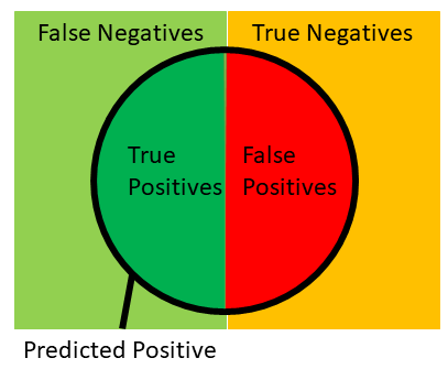
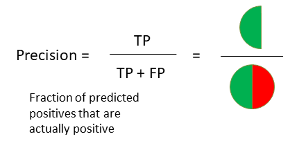
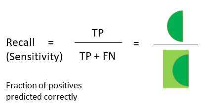
The datasets contains transactions made by credit cards in September 2013 by european cardholders.

This dataset presents transactions that occurred in two days, where we have 492 frauds out of 284,807 transactions.

The dataset is highly unbalanced, the positive class (frauds) account for 0.172% of all transactions.

It contains only numerical input variables which are the result of a PCA transformation.

Unfortunately, due to confidentiality issues, we cannot provide the original features and more background information about the data.

Features V1, V2, ... V28 are the principal components obtained with PCA, the only features which have not been transformed with PCA are 'Time' and 'Amount'.

Feature 'Time' contains the seconds elapsed between each transaction and the first transaction in the dataset. The feature 'Amount' is the transaction Amount, this feature can be used for example-dependant cost-senstive learning.

Feature 'Class' is the response variable and it takes value 1 in case of fraud and 0 otherwise.

Imports

import bhishan
from bhishan import bp

%load_ext autoreload
%autoreload 2

The autoreload extension is already loaded. To reload it, use:
  %reload_ext autoreload

import numpy as np
import pandas as pd
import seaborn as sns
sns.set(color_codes=True)
import scikitplot as skplot

import matplotlib
import matplotlib.pyplot as plt
%matplotlib inline

import os
import time

import scipy
from scipy import stats

import sklearn
from sklearn.model_selection import train_test_split
from sklearn import metrics
from scikitplot import metrics as skmetrics

# scale and split
from sklearn.preprocessing import MinMaxScaler, StandardScaler, RobustScaler
from sklearn.model_selection import train_test_split
from sklearn.model_selection import StratifiedKFold

# classifiers
from sklearn.ensemble import IsolationForest
from sklearn.neighbors import LocalOutlierFactor
from sklearn.svm import OneClassSVM

# random state
SEED = 0
RNG = np.random.RandomState(SEED)

# Jupyter notebook settings for pandas
pd.set_option('display.max_columns', 200)
pd.set_option('display.max_rows', 100) # None for all the rows
pd.set_option('display.max_colwidth', 50)

%load_ext watermark
%watermark -a "Bhishan Poudel" -d -v -m
%watermark -iv

The watermark extension is already loaded. To reload it, use:
  %reload_ext watermark
Bhishan Poudel 2020-09-28 

CPython 3.7.7
IPython 7.18.1

compiler   : Clang 4.0.1 (tags/RELEASE_401/final)
system     : Darwin
release    : 19.6.0
machine    : x86_64
processor  : i386
CPU cores  : 4
interpreter: 64bit
scikitplot 0.3.7
sklearn    0.23.1
seaborn    0.11.0
pandas     1.1.0
matplotlib 3.2.1
autopep8   1.5.2
json       2.0.9
bhishan    0.3.1
scipy      1.4.1
numpy      1.18.4

Useful Functions

def show_methods(obj, ncols=4):
    lst = [i for i in dir(obj) if i[0]!='_' ]
    df = pd.DataFrame(np.array_split(lst,ncols)).T.fillna('')
    return df

Load the data

df = pd.read_csv('../data/raw/creditcard.csv.zip',compression='zip')
print(df.shape)
df.head()

(284807, 31)

	Time	V1	V2	V3	V4	V5	V6	V7	V8	V9	V10	V11	V12	V13	V14	V15	V16	V17	V18	V19	V20	V21	V22	V23	V24	V25	V26	V27	V28	Amount	Class
0	0.0	-1.359807	-0.072781	2.536347	1.378155	-0.338321	0.462388	0.239599	0.098698	0.363787	0.090794	-0.551600	-0.617801	-0.991390	-0.311169	1.468177	-0.470401	0.207971	0.025791	0.403993	0.251412	-0.018307	0.277838	-0.110474	0.066928	0.128539	-0.189115	0.133558	-0.021053	149.62	0
1	0.0	1.191857	0.266151	0.166480	0.448154	0.060018	-0.082361	-0.078803	0.085102	-0.255425	-0.166974	1.612727	1.065235	0.489095	-0.143772	0.635558	0.463917	-0.114805	-0.183361	-0.145783	-0.069083	-0.225775	-0.638672	0.101288	-0.339846	0.167170	0.125895	-0.008983	0.014724	2.69	0
2	1.0	-1.358354	-1.340163	1.773209	0.379780	-0.503198	1.800499	0.791461	0.247676	-1.514654	0.207643	0.624501	0.066084	0.717293	-0.165946	2.345865	-2.890083	1.109969	-0.121359	-2.261857	0.524980	0.247998	0.771679	0.909412	-0.689281	-0.327642	-0.139097	-0.055353	-0.059752	378.66	0
3	1.0	-0.966272	-0.185226	1.792993	-0.863291	-0.010309	1.247203	0.237609	0.377436	-1.387024	-0.054952	-0.226487	0.178228	0.507757	-0.287924	-0.631418	-1.059647	-0.684093	1.965775	-1.232622	-0.208038	-0.108300	0.005274	-0.190321	-1.175575	0.647376	-0.221929	0.062723	0.061458	123.50	0
4	2.0	-1.158233	0.877737	1.548718	0.403034	-0.407193	0.095921	0.592941	-0.270533	0.817739	0.753074	-0.822843	0.538196	1.345852	-1.119670	0.175121	-0.451449	-0.237033	-0.038195	0.803487	0.408542	-0.009431	0.798278	-0.137458	0.141267	-0.206010	0.502292	0.219422	0.215153	69.99	0

Train test split with stratify

from sklearn.model_selection import train_test_split

target = 'Class'
Xtrain, Xtest, ytrain, ytest = train_test_split(
    df.drop(target,axis=1), df[target],
    test_size=0.2, random_state=SEED, stratify=df[target])

df.shape, Xtrain.shape, Xtest.shape

((284807, 31), (227845, 30), (56962, 30))

outlier_fraction = ytrain[ytrain==1].shape[0] /   ytrain[ytrain==0].shape[0]

Classification: isolationForest

Reference:
scikit learn
https://scikit-learn.org/stable/modules/outlier_detection.html

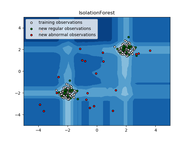
One efficient way of performing outlier detection in high-dimensional datasets is to use random forests. The ensemble.IsolationForest ‘isolates’ observations by randomly selecting a feature and then randomly selecting a split value between the maximum and minimum values of the selected feature.

Since recursive partitioning can be represented by a tree structure, the number of splittings required to isolate a sample is equivalent to the path length from the root node to the terminating node.

This path length, averaged over a forest of such random trees, is a measure of normality and our decision function.

Random partitioning produces noticeably shorter paths for anomalies. Hence, when a forest of random trees collectively produce shorter path lengths for particular samples, they are highly likely to be anomalies.

The implementation of ensemble.IsolationForest is based on an ensemble of tree.ExtraTreeRegressor. Following Isolation Forest original paper, the maximum depth of each tree is set to where is the number of samples used to build the tree (see (Liu et al., 2008) for more details).

This algorithm is illustrated below.

%%time

clf_iso = IsolationForest(n_estimators=100,
                      max_samples=len(Xtrain),
                      n_jobs=-1,
                      contamination=outlier_fraction,
                      random_state=SEED,
                      verbose=1)


# fitting  
clf_iso.fit(Xtrain)

# prediction
yprobs = clf_iso.decision_function(Xtest) # this is 1d array
ypreds = clf_iso.predict(Xtest)

# algorithm gives 1 and -1 classes, make them 0 and 1
ypreds[ypreds == 1] = 0
ypreds[ypreds == -1] = 1

ypreds_iso = ypreds

print(metrics.classification_report(ytest, ypreds_iso))

              precision    recall  f1-score   support

           0       1.00      1.00      1.00     56864
           1       0.26      0.29      0.27        98

    accuracy                           1.00     56962
   macro avg       0.63      0.64      0.64     56962
weighted avg       1.00      1.00      1.00     56962

df_eval = pd.DataFrame({
    'Model': [],
    'Description': [],
    'Accuracy': [],
    'Precision': [],
    'Recall': [],
    'F1 Weighted': [],
})

model_name = 'Isolation Forest'
desc = 'default'
sort_col = 'Recall'

acc = metrics.accuracy_score(ytest,ypreds_iso)
pre = metrics.precision_score(ytest,ypreds_iso)
rec = metrics.recall_score(ytest,ypreds_iso)
f1 = metrics.f1_score(ytest,ypreds_iso,average='weighted')

row = [ model_name,desc]
row = row + [acc, pre, rec, f1]
df_eval.loc[len(df_eval)] = row
df_eval = df_eval.drop_duplicates(subset=[ 'Model', 'Description'])
df_eval = df_eval.sort_values(sort_col,ascending=False)


display(df_eval.style.background_gradient(subset=[sort_col]))

	Model	Description	Accuracy	Precision	Recall	F1 Weighted
0	Isolation Forest	default	0.997384	0.261682	0.285714	0.997442

skmetrics.plot_confusion_matrix(ytest, ypreds_iso)

<matplotlib.axes._subplots.AxesSubplot at 0x7ff16d6dcdd0>

Classification: LOF (Local Outlier Factor)

Reference: sklearn

Unsupervised Outlier Detection using Local Outlier Factor (LOF)

The anomaly score of each sample is called Local Outlier Factor. It measures the local deviation of density of a given sample with respect to its neighbors. It is local in that the anomaly score depends on how isolated the object is with respect to the surrounding neighborhood. More precisely, locality is given by k-nearest neighbors, whose distance is used to estimate the local density. By comparing the local density of a sample to the local densities of its neighbors, one can identify samples that have a substantially lower density than their neighbors. These are considered outliers.

%%time

clf_lof = LocalOutlierFactor(n_neighbors=20,
                      algorithm='auto', 
                      leaf_size=30,
                      metric='minkowski',
                      p=2,
                      n_jobs=-1,
                      metric_params=None,
                      novelty=True,
                      contamination=outlier_fraction)

clf_lof.fit(Xtrain)
ypreds = clf_lof.predict(Xtest)

# alogrithm gives 1 and -1 classes, make them 0 and 1
ypreds[ypreds == 1] = 0
ypreds[ypreds == -1] = 1

ypreds_lof = ypreds

CPU times: user 11 s, sys: 223 ms, total: 11.3 s
Wall time: 4.34 s

print(metrics.classification_report(ytest, ypreds_lof))

              precision    recall  f1-score   support

           0       1.00      1.00      1.00     56864
           1       0.03      0.03      0.03        98

    accuracy                           1.00     56962
   macro avg       0.51      0.51      0.51     56962
weighted avg       1.00      1.00      1.00     56962

model_name = 'Local Outlier Factor'
desc = 'default'
sort_col = 'Recall'
ypreds = ypreds_lof

acc = metrics.accuracy_score(ytest,ypreds)
pre = metrics.precision_score(ytest,ypreds)
rec = metrics.recall_score(ytest,ypreds)
f1 = metrics.f1_score(ytest,ypreds,average='weighted')


row = [ model_name,desc]
row = row + [acc, pre, rec, f1]
df_eval.loc[len(df_eval)] = row
df_eval = df_eval.drop_duplicates(subset=[ 'Model', 'Description'])
df_eval = df_eval.sort_values(sort_col,ascending=False)


display(df_eval.style.background_gradient(subset=[sort_col]))

	Model	Description	Accuracy	Precision	Recall	F1 Weighted
0	Isolation Forest	default	0.997384	0.261682	0.285714	0.997442
1	Local Outlier Factor	default	0.996331	0.025641	0.030612	0.996493

skmetrics.plot_confusion_matrix(ytest, ypreds_lof)

<matplotlib.axes._subplots.AxesSubplot at 0x7ff15cd18510>

Classification Evaluation Metrics

show_methods(clf_iso)

	0	1	2	3
0	base_estimator	estimators_	max_samples	oob_score
1	base_estimator_	estimators_features_	max_samples_	predict
2	behaviour	estimators_samples_	n_estimators	random_state
3	bootstrap	fit	n_features_	score_samples
4	bootstrap_features	fit_predict	n_features_in_	set_params
5	contamination	get_params	n_jobs	verbose
6	decision_function	max_features	offset_	warm_start
7	estimator_params

show_methods(clf_lof)

	0	1	2	3
0	algorithm	get_params	n_jobs	offset_
1	contamination	kneighbors	n_neighbors	p
2	decision_function	kneighbors_graph	n_neighbors_	predict
3	effective_metric_	leaf_size	n_samples_fit_	radius
4	effective_metric_params_	metric	negative_outlier_factor_	score_samples
5	fit	metric_params	novelty	set_params
6	fit_predict	n_features_in_

help(clf_iso.decision_function)

Help on method decision_function in module sklearn.ensemble._iforest:

decision_function(X) method of sklearn.ensemble._iforest.IsolationForest instance
    Average anomaly score of X of the base classifiers.
    
    The anomaly score of an input sample is computed as
    the mean anomaly score of the trees in the forest.
    
    The measure of normality of an observation given a tree is the depth
    of the leaf containing this observation, which is equivalent to
    the number of splittings required to isolate this point. In case of
    several observations n_left in the leaf, the average path length of
    a n_left samples isolation tree is added.
    
    Parameters
    ----------
    X : {array-like, sparse matrix} of shape (n_samples, n_features)
        The input samples. Internally, it will be converted to
        ``dtype=np.float32`` and if a sparse matrix is provided
        to a sparse ``csr_matrix``.
    
    Returns
    -------
    scores : ndarray of shape (n_samples,)
        The anomaly score of the input samples.
        The lower, the more abnormal. Negative scores represent outliers,
        positive scores represent inliers.

yprobs_iso = clf_iso.decision_function(Xtest)
yprobs_iso.shape, yprobs_iso[:10]

((56962,),
 array([0.17929489, 0.18313638, 0.17685782, 0.18223546, 0.19401706,
        0.1876981 , 0.19039054, 0.17579801, 0.18324446, 0.17319798]))

yprobs_lof = clf_lof.decision_function(Xtest)
yprobs_lof.shape

(56962,)

skmetrics.plot_precision_recall(ytest, np.c_[yprobs_iso, 1 - yprobs_iso])

<matplotlib.axes._subplots.AxesSubplot at 0x7ff16d65f3d0>

skmetrics.plot_precision_recall(ytest, np.c_[yprobs_iso, 1 - yprobs_iso])

<matplotlib.axes._subplots.AxesSubplot at 0x7ff16da93190>