Table of Contents

• 1  Data Description
• 2  Imports
• 3  Useful Scripts
• 4  Load the data
• 5  descriptive statistics
  • 5.1  Mean
  • 5.2  standard deviation
  • 5.3  skewness
  • 5.4  kurtosis
• 6  Robust statistics: median
• 7  Outliers
• 8  Mutual Information (MI) between Target and the Predictors

Kernel Author:
Bhishan Poudel, Data Scientist, Ph.D Astrophysics .

Data Description

This dataset contains house sale prices for King County, which includes Seattle. It includes homes sold between May 2014 and May 2015.

• Dependent features: 1 (price)
• Features : 19 home features
• Id: 1 house ID

Task: Try to estimate the price based on given features.

Imports

import numpy as np
import pandas as pd
import seaborn as sns
sns.set(color_codes=True)

import matplotlib
import matplotlib.pyplot as plt
%matplotlib inline

import os
import time

# random state
SEED = 0
RNG = np.random.RandomState(SEED)

# Jupyter notebook settings for pandas
pd.set_option('display.max_columns', 200)
pd.set_option('display.max_rows', 100) # None for all the rows
pd.set_option('display.max_colwidth', 50)

print([(x.__name__,x.__version__) for x in [np, pd,sns,matplotlib]])

[('numpy', '1.16.4'), ('pandas', '0.25.0'), ('seaborn', '0.9.0'), ('matplotlib', '3.1.1')]

import scipy
from scipy import stats

import IPython
from IPython.display import display

from sklearn.preprocessing import MinMaxScaler, StandardScaler, RobustScaler

Useful Scripts

def show_method_attributes(method, ncols=7):
    """ Show all the attributes of a given method.
    Example:
    ========
    show_method_attributes(list)
     """
    x = [i for i in dir(method) if i[0].islower()]
    x = [i for i in x if i not in 'os np pd sys time psycopg2'.split()]

    return pd.DataFrame(np.array_split(x,ncols)).T.fillna('')

def json_dump_tofile(myjson,ofile,sort_keys=False):
    """Write json dictionary to a datafile.
    
    Usage:
    myjson = {'num': 5, my_list = [1,2,'apple']}
    json_dump_tofile(myjson, ofile)
    
    """
    import io
    import json

    with io.open(ofile, 'w', encoding='utf8') as fo:
        json_str = json.dumps(myjson,
                          indent=4,
                          sort_keys=sort_keys,
                          separators=(',', ': '),
                          ensure_ascii=False)
        fo.write(str(json_str))

Load the data

df = pd.read_csv('../data/raw/kc_house_data.csv')
df.head()

	id	date	price	bedrooms	bathrooms	sqft_living	sqft_lot	floors	waterfront	view	condition	grade	sqft_above	sqft_basement	yr_built	yr_renovated	zipcode	lat	long	sqft_living15	sqft_lot15
0	7129300520	20141013T000000	221900.0	3	1.00	1180	5650	1.0	0	0	3	7	1180	0	1955	0	98178	47.5112	-122.257	1340	5650
1	6414100192	20141209T000000	538000.0	3	2.25	2570	7242	2.0	0	0	3	7	2170	400	1951	1991	98125	47.7210	-122.319	1690	7639
2	5631500400	20150225T000000	180000.0	2	1.00	770	10000	1.0	0	0	3	6	770	0	1933	0	98028	47.7379	-122.233	2720	8062
3	2487200875	20141209T000000	604000.0	4	3.00	1960	5000	1.0	0	0	5	7	1050	910	1965	0	98136	47.5208	-122.393	1360	5000
4	1954400510	20150218T000000	510000.0	3	2.00	1680	8080	1.0	0	0	3	8	1680	0	1987	0	98074	47.6168	-122.045	1800	7503

df.columns

Index(['id', 'date', 'price', 'bedrooms', 'bathrooms', 'sqft_living',
       'sqft_lot', 'floors', 'waterfront', 'view', 'condition', 'grade',
       'sqft_above', 'sqft_basement', 'yr_built', 'yr_renovated', 'zipcode',
       'lat', 'long', 'sqft_living15', 'sqft_lot15'],
      dtype='object')

descriptive statistics

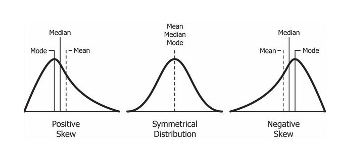
In statistics we sometimes are interested in the momentes of the variables. First four degrees of moments of a random variable has names: mean, variance, skewness, kurtosis and other moments are simply called moment of order n.

df.columns

Index(['id', 'date', 'price', 'bedrooms', 'bathrooms', 'sqft_living',
       'sqft_lot', 'floors', 'waterfront', 'view', 'condition', 'grade',
       'sqft_above', 'sqft_basement', 'yr_built', 'yr_renovated', 'zipcode',
       'lat', 'long', 'sqft_living15', 'sqft_lot15'],
      dtype='object')

features_sqft = df.filter(like='sqft').columns
features_sqft

Index(['sqft_living', 'sqft_lot', 'sqft_above', 'sqft_basement',
       'sqft_living15', 'sqft_lot15'],
      dtype='object')

Mean

def plot_statistics(df,features,statistic,color='b'):
    plt.figure(figsize=(12,4), dpi=80)
    sns.barplot(x=features, y= df[features].agg(statistic).sort_values(),color=color)
    plt.xlabel('Features')
    plt.ylabel(statistic.title())
    plt.title(statistic.title()+ ' for all features')
    plt.savefig(f'../reports/statistics/{statistic}.png',dpi=300)
    plt.xticks(rotation=90)
    plt.show()
    plt.close()

plot_statistics(df,features_sqft,'mean',color='b')
# mean is not zero, we need to normalize.

standard deviation

plot_statistics(df,features_sqft,'std',color='tomato')
# values are deviated, we need to normalize them.

skewness

• The third order moment is called skewness.
• Normal distribution has skewness of 0.
• If the skewness is less than 0, it is negatively skewed and has tail on left side.
• If the skewness is greater than 0, it is positively skewed and has tail on right side.

plot_statistics(df,features_sqft,'skew',color='seagreen')
# the features are skewed, we need to do boxcox transformation and
# also need to look at outliers.

feat = 'sqft_lot15'
df[feat].skew()

9.506743246764398

plt.figure(figsize=(12,4), dpi=80)
sns.distplot(df[feat], bins=300, kde=False)
plt.ylabel('Count')
plt.title(f'Distribution plot of feature: {feat}');

# almost all of data is centered around 0.

plt.figure(figsize=(12,4), dpi=80)
sns.distplot(df[feat], bins=9000, kde=False)
plt.ylabel('Count')
plt.title(f'Distribution plot of feature: {feat} with selected x limit')
plt.xlim(0,20_000)
plt.show()

# this does not look like gaussian.

plt.figure(figsize=(12,4), dpi=80)
sns.boxplot(df[feat])
plt.title(f'Box plot of feature: {feat}')
plt.savefig(f'../reports/statistics/{feat}_boxplot.png',dpi=300)

# there are so many outliers
# boxplot is hard to read, we can plot kurtosis plot.

kurtosis

• Kurtosis is related to the fourth moment.
• For Normal distribution, kurtosis has a value of 3.
• If kurtosis > 3 it is called lepto-kurtic and it has tall peak.
• If kurtosis < 3 it is called platy-kurtic and it is flat.
• If kurtosis = 3 it is called meso-kurtic. Normal curve is meso-kurtic.

plot_statistics(df,features_sqft,'kurtosis',color='darkorange')

df[feat].kurtosis()

150.76311004626973

Robust statistics: median

plot_statistics(df,features_sqft,'median',color='b')

# medians are not zero.

plt.figure(figsize=(12,4), dpi=80)
sns.barplot(x=features_sqft, y= (df[features_sqft].quantile(0.75)
            - df[features_sqft].quantile(0.25)).sort_values(), color='darkred')
plt.xlabel('Column')
plt.ylabel('IQR')
plt.title('Sqft features IQR')
plt.savefig('../reports/statistics/iqr.png',dpi=300)

plot_statistics(df,features_sqft,'std',color='darkred')
# iqr and std does not look similar, we may have outliers.

Outliers

plt.figure(figsize=(12,8))
ax = sns.boxplot(data = df[features_sqft], 
  orient = 'h', palette = 'winter')

ax.set(xlim=(-5,50_000))
ax.set_facecolor('#fafafa')
ax.set_title('Box plots of Sqft features')
ax.set_ylabel('Variables')
plt.savefig('../reports/statistics/boxplot_sqft_features.png',dpi=300)

Mutual Information (MI) between Target and the Predictors

• Mutual information (MI) between two random variables is a non-negative value, which measures the dependency between the variables.

• It is equal to zero if and only if two random variables are independent, and higher values mean higher dependency.

• Mutual Information is also known as information gain.

• Mutual information can be used as a criterion for feature selection and feature transformations in machine learning. It can be used to characterize both the relevance and redundancy of variables, such as the minimum redundancy feature selection.

from sklearn.feature_selection import mutual_info_classif

df.columns

Index(['id', 'date', 'price', 'bedrooms', 'bathrooms', 'sqft_living',
       'sqft_lot', 'floors', 'waterfront', 'view', 'condition', 'grade',
       'sqft_above', 'sqft_basement', 'yr_built', 'yr_renovated', 'zipcode',
       'lat', 'long', 'sqft_living15', 'sqft_lot15'],
      dtype='object')

all_features = df.columns.difference(['id','date','price'])
all_features

Index(['bathrooms', 'bedrooms', 'condition', 'floors', 'grade', 'lat', 'long',
       'sqft_above', 'sqft_basement', 'sqft_living', 'sqft_living15',
       'sqft_lot', 'sqft_lot15', 'view', 'waterfront', 'yr_built',
       'yr_renovated', 'zipcode'],
      dtype='object')

%%time
target = 'price'

mutual_infos = pd.Series(data=mutual_info_classif(df[all_features], df[target],
                                                  discrete_features=False,
                                                  random_state=SEED),
                         index=all_features)

CPU times: user 21.3 s, sys: 2.75 s, total: 24.1 s
Wall time: 24.2 s

mutual_infos.sort_values(ascending=False).to_frame()

	0
floors	0.569917
grade	0.509087
lat	0.333617
sqft_living	0.324773
bedrooms	0.289373
bathrooms	0.284329
sqft_living15	0.248312
zipcode	0.233668
sqft_above	0.213384
condition	0.201436
long	0.076660
sqft_lot15	0.075715
yr_built	0.070296
sqft_basement	0.065090
sqft_lot	0.061365
view	0.045477
yr_renovated	0.003725
waterfront	0.000000