Introduction to RNN and LSTM
References:
- https://www.kaggle.com/thebrownviking20/intro-to-recurrent-neural-networks-lstm-gru
- https://www.youtube.com/watch?v=UNmqTiOnRfg&t=3s
- https://medium.com/deep-math-machine-learning-ai/chapter-10-1-deepnlp-lstm-long-short-term-memory-networks-with-math-21477f8e4235
- https://machinelearningmastery.com/how-to-develop-lstm-models-for-time-series-forecasting/
- https://machinelearningmastery.com/time-series-prediction-lstm-recurrent-neural-networks-python-keras/ Recurrent Neural Networks
In a recurrent neural network we store the output activations from one or more of the layers of the network. Often these are hidden later activations. Then, the next time we feed an input example to the network, we include the previously-stored outputs as additional inputs. You can think of the additional inputs as being concatenated to the end of the “normal” inputs to the previous layer. For example, if a hidden layer had 10 regular input nodes and 128 hidden nodes in the layer, then it would actually have 138 total inputs (assuming you are feeding the layer’s outputs into itself à la Elman) rather than into another layer). Of course, the very first time you try to compute the output of the network you’ll need to fill in those extra 128 inputs with 0s or something.

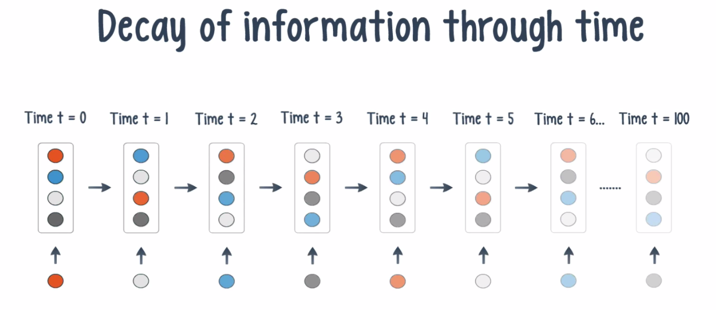
Now, even though RNNs are quite powerful, they suffer from Vanishing gradient problem which hinders them from using long term information, like they are good for storing memory 3-4 instances of past iterations but larger number of instances don't provide good results so we don't just use regular RNNs. Instead, we use a better variation of RNNs: Long Short Term Networks(LSTM).
What is Vanishing Gradient problem?
Vanishing gradient problem is a difficulty found in training artificial neural networks with gradient-based learning methods and backpropagation. In such methods, each of the neural network's weights receives an update proportional to the partial derivative of the error function with respect to the current weight in each iteration of training. The problem is that in some cases, the gradient will be vanishingly small, effectively preventing the weight from changing its value. In the worst case, this may completely stop the neural network from further training. As one example of the problem cause, traditional activation functions such as the hyperbolic tangent function have gradients in the range (0, 1), and backpropagation computes gradients by the chain rule. This has the effect of multiplying n of these small numbers to compute gradients of the "front" layers in an n-layer network, meaning that the gradient (error signal) decreases exponentially with n while the front layers train very slowly.

Long Short Term Memory(LSTM)
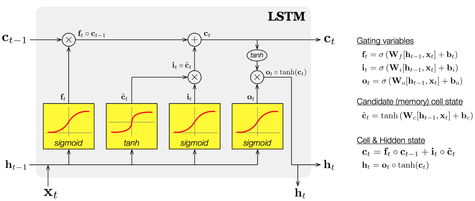
Long short-term memory (LSTM) units (or blocks) are a building unit for layers of a recurrent neural network (RNN). A RNN composed of LSTM units is often called an LSTM network. A common LSTM unit is composed of a cell, an input gate, an output gate and a forget gate. The cell is responsible for "remembering" values over arbitrary time intervals; hence the word "memory" in LSTM. Each of the three gates can be thought of as a "conventional" artificial neuron, as in a multi-layer (or feedforward) neural network: that is, they compute an activation (using an activation function) of a weighted sum. Intuitively, they can be thought as regulators of the flow of values that goes through the connections of the LSTM; hence the denotation "gate". There are connections between these gates and the cell.
The expression long short-term refers to the fact that LSTM is a model for the short-term memory which can last for a long period of time. An LSTM is well-suited to classify, process and predict time series given time lags of unknown size and duration between important events. LSTMs were developed to deal with the exploding and vanishing gradient problem when training traditional RNNs.

Components of LSTMs
So the LSTM cell contains the following components
- Forget Gate “f” ( a neural network with sigmoid)
- Candidate layer “C"(a NN with Tanh)
- Input Gate “I” ( a NN with sigmoid )
- Output Gate “O”( a NN with sigmoid)
- Hidden state “H” ( a vector )
Memory state “C” ( a vector)
Inputs to the LSTM cell at any step are Xt (current input) , Ht-1 (previous hidden state ) and Ct-1 (previous memory state).
Outputs from the LSTM cell are Ht (current hidden state ) and Ct (current memory state)
Working of gates in LSTMs
First, LSTM cell takes the previous memory state Ct-1 and does element wise multiplication with forget gate (f) to decide if present memory state Ct. If forget gate value is 0 then previous memory state is completely forgotten else f forget gate value is 1 then previous memory state is completely passed to the cell ( Remember f gate gives values between 0 and 1 ).
Ct = Ct-1 * ft
Calculating the new memory state:
Ct = Ct + (It * C`t)
Now, we calculate the output:
Ht = tanh(Ct)